---
title: "Bank runs as a coordination game — the Diamond-Dybvig model"
description: "Model bank runs as a coordination game using the Diamond-Dybvig framework in R, showing the Stag Hunt structure, deposit insurance as equilibrium selection, and contagion dynamics with N depositors."
author: "Raban Heller"
date: 2026-05-08
date-modified: 2026-05-08
categories:
- classical-games
- coordination
- bank-runs
- financial-economics
keywords: ["bank run", "Diamond-Dybvig", "coordination game", "Stag Hunt", "deposit insurance", "financial crisis", "contagion"]
labels: ["canonical-games", "coordination-games"]
tier: 1
bibliography: ../../../references.bib
vgwort: "TODO_VGWORT_classical-games_bank-runs-coordination"
image: thumbnail.png
image-alt: "Payoff matrix for the bank run coordination game showing efficient and bank-run equilibria"
citation:
type: webpage
url: https://r-heller.github.io/equilibria/tutorials/classical-games/bank-runs-coordination/
license: "CC BY-SA 4.0"
draft: false
has_static_fig: true
has_interactive_fig: true
has_shiny_app: false
---
```{r}
#| label: setup
#| include: false
library(ggplot2)
library(dplyr)
library(tidyr)
library(plotly)
okabe_ito <- c("#E69F00", "#56B4E9", "#009E73", "#F0E442",
"#0072B2", "#D55E00", "#CC79A7", "#999999")
theme_publication <- function(base_size = 12) {
theme_minimal(base_size = base_size) +
theme(
plot.title = element_text(size = base_size * 1.2, face = "bold"),
plot.subtitle = element_text(size = base_size * 0.9, color = "grey40"),
axis.line = element_line(color = "grey30", linewidth = 0.3),
panel.grid.minor = element_blank(),
legend.position = "bottom",
plot.margin = margin(10, 10, 10, 10)
)
}
```
## Introduction & motivation
Bank runs are among the most dramatic events in financial history. From the Great Depression bank panics of the 1930s to the Northern Rock run in 2007 and the Silicon Valley Bank collapse in 2023, the same fundamental dynamic recurs: depositors rush to withdraw their funds because they fear the bank will become insolvent -- and the very act of mass withdrawal causes the insolvency they feared. This self-fulfilling prophecy is a textbook example of a **coordination failure** and was formalised by Diamond and Dybvig (1983) in one of the most influential models in financial economics.
The Diamond-Dybvig model captures the essential tension in banking: banks transform short-term deposits into long-term illiquid investments (mortgages, business loans). This maturity transformation creates value -- long-term investments earn higher returns than short-term deposits -- but also creates **fragility**. If all depositors wait patiently until the investment matures, everyone earns the high return. But if too many depositors withdraw early, the bank must liquidate its illiquid assets at a loss, and there may not be enough to pay everyone. Each depositor therefore faces a strategic decision: wait (cooperate) or withdraw early (run). If you believe others will wait, you should wait too and enjoy the high return. But if you believe others will run, you should also run to avoid being the last one left with nothing.
This strategic structure is precisely that of a **Stag Hunt** -- a coordination game with two pure-strategy Nash equilibria. The efficient equilibrium (all wait) Pareto-dominates the bank-run equilibrium (all withdraw), but the bank-run equilibrium is **risk-dominant** when the liquidation value is sufficiently low relative to the promised return. The beauty of the Diamond-Dybvig framework is that it explains not only why bank runs happen, but also why **deposit insurance** works: by guaranteeing depositors their money regardless of others' actions, deposit insurance eliminates the strategic uncertainty that makes runs rational, converting the game from a coordination problem into one with a unique dominant strategy (wait). This tutorial implements the two-depositor version, extends it to $N$ depositors with contagion dynamics, and shows how institutional design -- deposit insurance, suspension of convertibility, and lender-of-last-resort facilities -- can eliminate the bad equilibrium.
## Mathematical formulation
Consider a bank with two depositors, each depositing $D = 1$. The bank invests in a long-term asset that returns $R > 1$ at maturity. If liquidated early, it yields only $L < 1$ per unit (fire-sale discount).
Each depositor chooses **Wait** (W) or **Withdraw** (X). Payoffs:
$$
\begin{array}{c|cc}
& \text{Wait} & \text{Withdraw} \\ \hline
\text{Wait} & R, \; R & 2L - 1, \; 1 \\
\text{Withdraw} & 1, \; 2L - 1 & L, \; L
\end{array}
$$
When both wait, the investment matures and each receives $R$. When both withdraw early, the bank liquidates for $2L$ total and each gets $L$. When one waits and one withdraws, the withdrawer gets their full deposit $D = 1$ (first-come-first-served), and the waiter gets the remaining liquidation value $2L - 1$.
**Equilibrium analysis** (assuming $R > 1 > L > 1/2$):
- **(Wait, Wait)** is a NE: given the other waits, $R > 1$ so waiting is a best response.
- **(Withdraw, Withdraw)** is a NE: given the other withdraws, $L > 2L - 1$ (since $L < 1$), so withdrawing is a best response.
- **Mixed NE**: Each deposits with probability $p^* = \frac{1 - L}{R - 2L + 1}$.
**Risk dominance**: The bank-run equilibrium risk-dominates when $L < \frac{R+1}{2R+2}$, i.e., when the liquidation value is sufficiently low. With deposit insurance (government guarantees $D = 1$ regardless), the payoff for waiting when the other withdraws becomes $1$ instead of $2L - 1$, making Wait strictly dominant and eliminating the run equilibrium.
**N-depositor extension**: With $N$ depositors, the bank liquidates if $k$ depositors withdraw. Each withdrawer gets $\min(1, NL/k)$, each waiter gets $\max(0, (NL - k) \cdot R / (N - k))$ if partial liquidation, or the full return $R$ if no liquidation occurs.
## R implementation
```{r}
#| label: bank-run-analysis
# Two-depositor Diamond-Dybvig game
bank_run_2player <- function(R, L) {
  stopifnot(R > 1, L < 1, L > 0.5)

  # Payoff matrix: [row action, col action]
  # Actions: 1 = Wait, 2 = Withdraw
  payoff1 <- matrix(c(R, 1, 2*L - 1, L), nrow = 2, byrow = TRUE,
                     dimnames = list(c("Wait", "Withdraw"), c("Wait", "Withdraw")))
  payoff2 <- t(payoff1)  # Symmetric game

  # Mixed NE probability of waiting
  # Player waits if: p*R + (1-p)*(2L-1) > p*1 + (1-p)*L
  # => p*(R-1) > (1-p)*(L - 2L + 1) = (1-p)*(1-L)
  # => p*(R-1) > (1-L) - p*(1-L)
  # => p*(R - 2L + 1 - 1 + 1) > 1 - L  ... simplify
  p_star <- (1 - L) / (R - 2*L + 1)

  # Risk dominance: (W,W) risk-dominates if (R - 1)(R - (2L-1)) > (1 - L)(L - (2L-1))
  rd_left <- (R - 1) * (R - (2*L - 1))
  rd_right <- (1 - L) * (L - (2*L - 1))
  wait_risk_dominates <- rd_left > rd_right

  list(payoff1 = payoff1, payoff2 = payoff2, p_star = p_star,
       wait_risk_dominates = wait_risk_dominates, R = R, L = L)
}

cat("=== Diamond-Dybvig Bank Run (R=1.5, L=0.7) ===\n")
game <- bank_run_2player(R = 1.5, L = 0.7)
cat("Payoff matrix (Player 1):\n")
print(game$payoff1)
cat(sprintf("\nMixed NE: Probability of waiting = %.3f\n", game$p_star))
cat(sprintf("(Wait, Wait) risk-dominates: %s\n", game$wait_risk_dominates))
cat("\n=== Low liquidation value (R=1.5, L=0.55) ===\n")
game2 <- bank_run_2player(R = 1.5, L = 0.55)
cat("Payoff matrix (Player 1):\n")
print(game2$payoff1)
cat(sprintf("Mixed NE: p* = %.3f\n", game2$p_star))
cat(sprintf("(Wait, Wait) risk-dominates: %s\n", game2$wait_risk_dominates))
# Deposit insurance: change payoff for (Wait, Withdraw) from (2L-1) to 1
cat("\n=== With deposit insurance (R=1.5, L=0.7) ===\n")
insured_payoff <- game$payoff1
insured_payoff["Wait", "Withdraw"] <- 1  # Government guarantees deposit
cat("Insured payoff matrix:\n")
print(insured_payoff)
cat("Wait is now strictly dominant: Wait payoff >= Withdraw payoff for both opponent actions\n")
cat(sprintf("  vs Wait:     %.2f (wait) vs %.2f (withdraw) -> %s\n",
            insured_payoff["Wait", "Wait"], insured_payoff["Withdraw", "Wait"],
            ifelse(insured_payoff["Wait", "Wait"] >= insured_payoff["Withdraw", "Wait"], "Wait wins", "Withdraw wins")))
cat(sprintf("  vs Withdraw: %.2f (wait) vs %.2f (withdraw) -> %s\n",
            insured_payoff["Wait", "Withdraw"], insured_payoff["Withdraw", "Withdraw"],
            ifelse(insured_payoff["Wait", "Withdraw"] >= insured_payoff["Withdraw", "Withdraw"], "Wait wins", "Withdraw wins")))
# N-depositor simulation
cat("\n=== N-Depositor Contagion Simulation ===\n")
simulate_bank_run <- function(N, R, L, initial_runners, rounds = 20) {
  # Each depositor has a panic threshold: they run if fraction of runners exceeds threshold
  set.seed(42)
  thresholds <- runif(N, 0.1, 0.9)  # Heterogeneous panic thresholds

  run_status <- rep(FALSE, N)
  # Initial runners (exogenous shock)
  run_status[sample(N, initial_runners)] <- TRUE

  history <- numeric(rounds)
  for (t in 1:rounds) {
    frac_running <- mean(run_status)
    history[t] <- frac_running
    # Non-runners check if they should panic
    for (i in which(!run_status)) {
      if (frac_running > thresholds[i]) {
        run_status[i] <- TRUE
      }
    }
  }
  history
}

N <- 100
for (init in c(5, 15, 30)) {
  hist <- simulate_bank_run(N, R = 1.5, L = 0.7, initial_runners = init)
  cat(sprintf("Initial runners: %2d/%d -> Final runners: %.0f/%d (%.0f%%)\n",
              init, N, hist[length(hist)] * N, N, 100 * hist[length(hist)]))
}
```
## Static publication-ready figure
```{r}
#| label: fig-bank-run-contagion
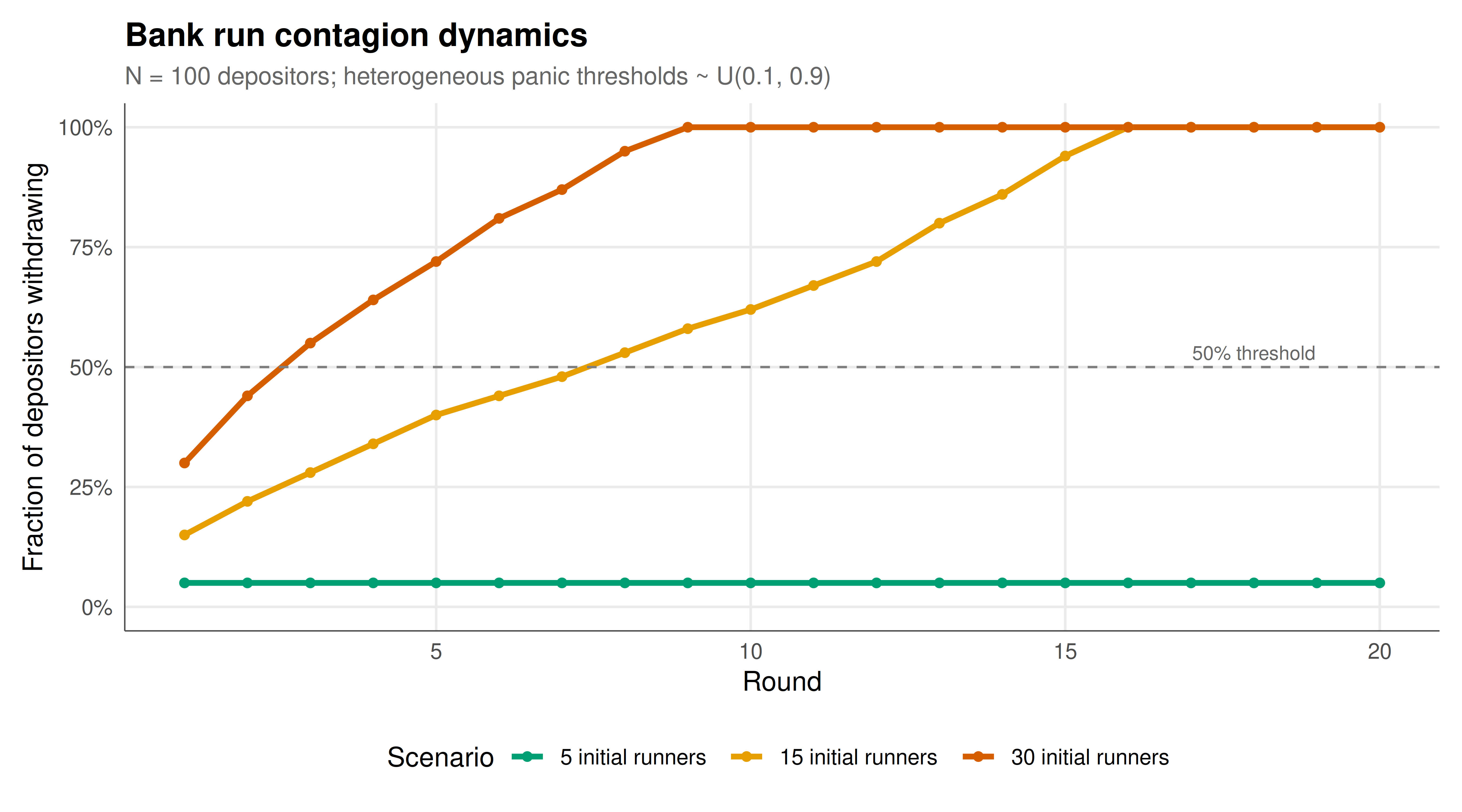
#| fig-cap: "Figure 1. Bank run contagion dynamics for N = 100 depositors with heterogeneous panic thresholds. Three scenarios show how the initial shock size determines whether a run cascades. With 5 initial runners, contagion is contained; with 15, a partial run develops; with 30, a full bank run engulfs the system. The tipping point illustrates the coordination failure inherent in the Diamond-Dybvig model. Okabe-Ito palette."
#| dev: [png, pdf]
#| fig-width: 9
#| fig-height: 5
#| dpi: 300
N <- 100
rounds <- 20

contagion_data <- bind_rows(
  lapply(c(5, 15, 30), function(init) {
    hist <- simulate_bank_run(N, R = 1.5, L = 0.7,
                               initial_runners = init, rounds = rounds)
    tibble(
      round = 1:rounds,
      fraction_running = hist,
      initial = sprintf("%d initial runners", init)
    )
  })
)

contagion_data$initial <- factor(contagion_data$initial,
                                  levels = c("5 initial runners",
                                            "15 initial runners",
                                            "30 initial runners"))

p_contagion <- ggplot(contagion_data, aes(x = round, y = fraction_running,
                                           color = initial)) +
  geom_line(linewidth = 1.2) +
  geom_point(size = 1.5) +
  geom_hline(yintercept = 0.5, linetype = "dashed", color = "grey50", linewidth = 0.5) +
  annotate("text", x = 18, y = 0.53, label = "50% threshold", size = 3, color = "grey40") +
  scale_color_manual(values = okabe_ito[c(3, 1, 6)], name = "Scenario") +
  scale_y_continuous(labels = scales::percent_format(accuracy = 1),
                     limits = c(0, 1)) +
  labs(
    title = "Bank run contagion dynamics",
    subtitle = "N = 100 depositors; heterogeneous panic thresholds ~ U(0.1, 0.9)",
    x = "Round", y = "Fraction of depositors withdrawing"
  ) +
  theme_publication()

p_contagion
```
## Interactive figure
```{r}
#| label: fig-bank-run-parameter
# How the mixed NE probability varies with R and L
param_grid <- expand.grid(
  R = seq(1.1, 2.5, by = 0.05),
  L = seq(0.51, 0.95, by = 0.02)
) |>
  filter(R > 1, L > 0.5, L < 1) |>
  mutate(
    p_star = (1 - L) / (R - 2*L + 1),
    p_star = pmin(pmax(p_star, 0), 1),  # Clamp to [0,1]
    rd_left = (R - 1) * (R - (2*L - 1)),
    rd_right = (1 - L) * (L - (2*L - 1)),
    risk_dom = ifelse(rd_left > rd_right, "Wait", "Withdraw"),
    text = paste0("R = ", R, ", L = ", L,
                  "\np(Wait) = ", round(p_star, 3),
                  "\nRisk dominant: ", risk_dom)
  )

p_param <- ggplot(param_grid, aes(x = R, y = L, fill = p_star, text = text)) +
  geom_tile() +
  scale_fill_gradient2(
    low = okabe_ito[6], mid = okabe_ito[1], high = okabe_ito[3],
    midpoint = 0.5,
    name = "p(Wait)\nin mixed NE",
    limits = c(0, 1)
  ) +
  labs(
    title = "Mixed NE probability of waiting across parameter space",
    subtitle = "Higher R (return) and higher L (liquidation value) encourage waiting",
    x = "Investment return (R)", y = "Liquidation value (L)"
  ) +
  theme_publication()

ggplotly(p_param, tooltip = "text") |>
  config(displaylogo = FALSE,
         modeBarButtonsToRemove = c("select2d", "lasso2d"))
```
## Interpretation
The Diamond-Dybvig model reveals that bank runs are not necessarily caused by fundamental insolvency but can emerge as a **self-fulfilling coordination failure** among perfectly rational depositors. The two-depositor game makes the structure transparent: both (Wait, Wait) and (Withdraw, Withdraw) are Nash equilibria, and the bank-run equilibrium can be risk-dominant when liquidation values are low relative to promised returns. The parameter sweep shows that the mixed-strategy equilibrium probability of waiting increases with both the investment return $R$ (making patience more attractive) and the liquidation value $L$ (making early withdrawal less costly, which paradoxically also reduces the fear of being the last to withdraw).
The N-depositor contagion simulation demonstrates a crucial feature of real bank runs: **nonlinear cascading**. With heterogeneous panic thresholds among depositors, a small initial shock (5 runners out of 100) can be absorbed without triggering a cascade, while a moderately larger shock (30 runners) pushes the system past a tipping point where panic feeds on itself until nearly all depositors have withdrawn. This tipping-point behaviour explains the sudden, explosive nature of real bank runs -- the system appears stable until it suddenly is not.
Deposit insurance resolves the coordination failure by changing the game structure rather than changing depositor preferences. By guaranteeing each depositor's principal regardless of others' behaviour, deposit insurance makes Wait a strictly dominant strategy, eliminating the bank-run equilibrium entirely. This explains why deposit insurance, first introduced in the United States through the FDIC in 1933, has been so effective at preventing classic retail bank runs -- though it introduces moral hazard on the bank's side, which requires complementary regulation. The model also illuminates why wholesale bank runs (among institutional creditors not covered by insurance, as in the 2008 financial crisis) remain a persistent threat. The fundamental tension between maturity transformation and coordination fragility is structural, not behavioural, and requires institutional solutions rather than appeals to calm.
## Extensions & related tutorials
- [The Stag Hunt — coordination, trust, and risk dominance](../stag-hunt/) -- the abstract coordination game underlying bank runs.
- [Global games and coordination under private information](../../bayesian-methods/global-games-coordination/) -- how private signals resolve multiplicity in bank-run models.
- [Signaling games and perfect Bayesian equilibrium](../../foundations/signaling-games-pbe/) -- central bank communication as a signal to prevent runs.
- [Nash equilibrium in mixed strategies](../../foundations/nash-equilibrium-mixed/) -- the mixed equilibrium computation used here.
- [Folk theorem and sustained cooperation](../../foundations/folk-theorem-perfect-monitoring/) -- repeated interaction and trust-building in banking relationships.
## References
::: {#refs}
:::