---
title: "Chicken / Hawk-Dove — brinkmanship and anti-coordination"
description: "Analyse the Chicken (Hawk-Dove) game in R, computing pure and mixed Nash equilibria, exploring the evolutionary stable strategy, and connecting to models of escalation and conflict."
author: "Raban Heller"
date: 2026-05-08
date-modified: 2026-05-08
categories:
- classical-games
- chicken
- hawk-dove
- anti-coordination
- ess
keywords: ["Chicken", "Hawk-Dove", "anti-coordination", "brinkmanship", "ESS", "escalation"]
labels: ["canonical-games", "conflict-games"]
tier: 1
bibliography: ../../../references.bib
vgwort: "TODO_VGWORT_classical-games_chicken-hawk-dove"
image: thumbnail.png
image-alt: "Phase diagram of Hawk-Dove game showing ESS and population dynamics"
citation:
type: webpage
url: https://r-heller.github.io/equilibria/tutorials/classical-games/chicken-hawk-dove/
license: "CC BY-SA 4.0"
draft: false
has_static_fig: true
has_interactive_fig: true
has_shiny_app: false
---
```{r}
#| label: setup
#| include: false
library(ggplot2)
library(dplyr)
library(tidyr)
library(plotly)
okabe_ito <- c("#E69F00", "#56B4E9", "#009E73", "#F0E442",
"#0072B2", "#D55E00", "#CC79A7", "#999999")
theme_publication <- function(base_size = 12) {
theme_minimal(base_size = base_size) +
theme(
plot.title = element_text(size = base_size * 1.2, face = "bold"),
plot.subtitle = element_text(size = base_size * 0.9, color = "grey40"),
axis.line = element_line(color = "grey30", linewidth = 0.3),
panel.grid.minor = element_blank(),
legend.position = "bottom",
plot.margin = margin(10, 10, 10, 10)
)
}
```
## Introduction & motivation
The game of Chicken — known in evolutionary biology as the **Hawk-Dove game** (@maynard_smith_1982) — models situations where two parties escalate toward a catastrophic outcome unless one backs down. In the classic narrative, two drivers race toward each other; the first to swerve is the "chicken" (loses face but survives), while if neither swerves, both crash. The game has two asymmetric pure Nash equilibria (one swerves, the other doesn't) and one symmetric mixed equilibrium where each player randomises between toughness and concession. Unlike the Prisoner's Dilemma, there is no dominant strategy — the best action depends on what the opponent does. Unlike the Stag Hunt, the pure equilibria are asymmetric, creating a distributional conflict about who concedes. The Hawk-Dove framing adds biological insight: Hawks always fight for a resource (value $V$) but risk injury (cost $C$); Doves share or retreat. When $C > V$, the mixed ESS has both types coexisting in the population at frequency $p^* = V/C$, explaining why aggression and concession coexist in nature. This game underlies models of nuclear brinkmanship, labour disputes, territorial contests, and any situation where mutual toughness is the worst outcome for everyone.
## Mathematical formulation
The Hawk-Dove payoff matrix with resource value $V$ and fighting cost $C$ ($C > V > 0$):
$$
\begin{array}{c|cc}
& \text{Hawk} & \text{Dove} \\ \hline
\text{Hawk} & \frac{V-C}{2}, \frac{V-C}{2} & V, 0 \\
\text{Dove} & 0, V & \frac{V}{2}, \frac{V}{2}
\end{array}
$$
**Pure NE**: (Hawk, Dove) with payoffs $(V, 0)$ and (Dove, Hawk) with payoffs $(0, V)$ — asymmetric.
**Mixed NE / ESS**: Each plays Hawk with probability $p^* = V/C$. Expected payoff: $V(C-V)/(2C)$ — less than the Dove-Dove outcome of $V/2$ but better than the Hawk-Hawk disaster.
The mixed NE is the unique **evolutionarily stable strategy** (ESS): a population at $p^* = V/C$ cannot be invaded by a small group of pure Hawks or pure Doves.
## R implementation
```{r}
#| label: hawk-dove-analysis
hawk_dove <- function(V, C) {
  stopifnot(C > V, V > 0)

  p_star <- V / C  # ESS frequency of Hawk
  payoff_hh <- (V - C) / 2
  payoff_hd <- V
  payoff_dh <- 0
  payoff_dd <- V / 2

  # Expected payoff at ESS
  eu_ess <- p_star * payoff_hh + (1 - p_star) * payoff_hd
  # = V/C * (V-C)/2 + (1-V/C) * V
  # = V(V-C)/(2C) + V(C-V)/C = V(V-C+2C-2V)/(2C) = V(C-V)/(2C)

  list(
    V = V, C = C, p_star = p_star,
    payoff_matrix = matrix(c(payoff_hh, payoff_dh, payoff_hd, payoff_dd), nrow = 2,
                            dimnames = list(c("Hawk","Dove"), c("Hawk","Dove"))),
    eu_ess = eu_ess,
    eu_dd = payoff_dd
  )
}

cat("=== Hawk-Dove Game (V=2, C=6) ===\n")
hd <- hawk_dove(2, 6)
cat("Payoff matrix:\n"); print(hd$payoff_matrix)
cat(sprintf("\nESS: p* = %.3f (%.1f%% Hawks)\n", hd$p_star, 100 * hd$p_star))
cat(sprintf("Expected payoff at ESS: %.3f\n", hd$eu_ess))
cat(sprintf("Dove-Dove payoff: %.3f (Pareto-superior but not stable)\n", hd$eu_dd))
cat("\n=== Low-cost conflict (V=2, C=3) ===\n")
hd2 <- hawk_dove(2, 3)
cat(sprintf("ESS: p* = %.3f (%.1f%% Hawks — more aggression when cost is lower)\n",
            hd2$p_star, 100 * hd2$p_star))
cat("\n=== High-cost conflict (V=2, C=20) ===\n")
hd3 <- hawk_dove(2, 20)
cat(sprintf("ESS: p* = %.3f (%.1f%% Hawks — deterred by high cost)\n",
            hd3$p_star, 100 * hd3$p_star))
```
## Static publication-ready figure
```{r}
#| label: fig-hawk-dove-ess
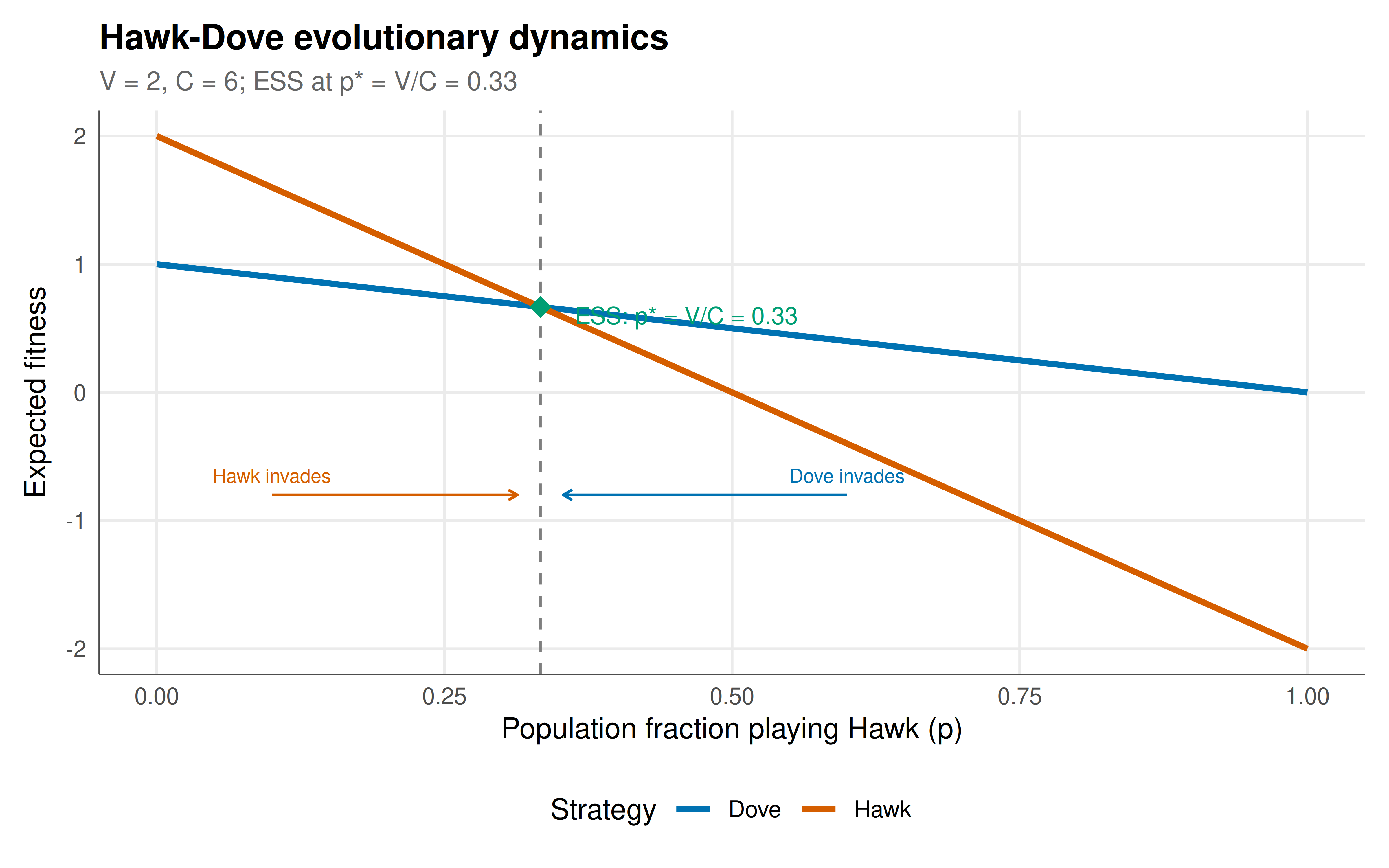
#| fig-cap: "Figure 1. Evolutionary dynamics of the Hawk-Dove game (V=2, C=6). Top: fitness of Hawk vs Dove as a function of population Hawk frequency p. The ESS occurs at p* = V/C = 1/3 where fitnesses are equal. Below p*, Hawks earn more (Hawk frequency increases); above p*, Doves earn more (Hawk frequency decreases). Bottom: the ESS frequency V/C as a function of the cost-to-value ratio C/V. Higher conflict costs drive the population toward more Doves. Okabe-Ito palette."
#| dev: [png, pdf]
#| fig-width: 8
#| fig-height: 5
#| dpi: 300
V <- 2; C <- 6
p_seq <- seq(0, 1, by = 0.005)

fitness_data <- tibble(
  p = p_seq,
  fitness_hawk = p * (V - C)/2 + (1 - p) * V,
  fitness_dove = p * 0 + (1 - p) * V/2
)

fitness_long <- fitness_data |>
  pivot_longer(-p, names_to = "strategy", values_to = "fitness") |>
  mutate(strategy = ifelse(strategy == "fitness_hawk", "Hawk", "Dove"))

p_ess <- ggplot(fitness_long, aes(x = p, y = fitness, color = strategy)) +
  geom_line(linewidth = 1.2) +
  geom_vline(xintercept = V/C, linetype = "dashed", color = "grey50") +
  geom_point(aes(x = V/C, y = V * (C - V) / (2 * C)), color = okabe_ito[3],
             size = 4, shape = 18, inherit.aes = FALSE) +
  annotate("text", x = V/C + 0.03, y = 0.6,
           label = sprintf("ESS: p* = V/C = %.2f", V/C),
           size = 3.5, hjust = 0, color = okabe_ito[3]) +
  annotate("segment", x = 0.1, y = -0.8, xend = V/C - 0.02, yend = -0.8,
           arrow = arrow(length = unit(0.15, "cm")), color = okabe_ito[6]) +
  annotate("text", x = 0.1, y = -0.65, label = "Hawk invades", size = 2.8, color = okabe_ito[6]) +
  annotate("segment", x = 0.6, y = -0.8, xend = V/C + 0.02, yend = -0.8,
           arrow = arrow(length = unit(0.15, "cm")), color = okabe_ito[5]) +
  annotate("text", x = 0.6, y = -0.65, label = "Dove invades", size = 2.8, color = okabe_ito[5]) +
  scale_color_manual(values = c(Hawk = okabe_ito[6], Dove = okabe_ito[5]),
                      name = "Strategy") +
  labs(
    title = "Hawk-Dove evolutionary dynamics",
    subtitle = sprintf("V = %d, C = %d; ESS at p* = V/C = %.2f", V, C, V/C),
    x = "Population fraction playing Hawk (p)", y = "Expected fitness"
  ) +
  theme_publication()

p_ess
```
## Interactive figure
```{r}
#| label: fig-hawk-dove-vc-interactive
# ESS hawk frequency as function of V and C
vc_grid <- expand.grid(V = seq(1, 10, by = 0.5), C = seq(2, 20, by = 0.5)) |>
  filter(C > V) |>
  mutate(
    p_star = V / C,
    text = paste0("V = ", V, ", C = ", C,
                  "\np*(Hawk) = ", round(p_star, 3),
                  "\nConflict severity: C/V = ", round(C/V, 1))
  )

p_vc <- ggplot(vc_grid, aes(x = V, y = C, fill = p_star, text = text)) +
  geom_tile() +
  scale_fill_gradient2(low = okabe_ito[5], mid = okabe_ito[4], high = okabe_ito[6],
                        midpoint = 0.5, name = "ESS Hawk freq") +
  labs(
    title = "ESS Hawk frequency across resource value and conflict cost",
    subtitle = "Higher V/C ratio → more aggression; lower → more accommodation",
    x = "Resource value (V)", y = "Conflict cost (C)"
  ) +
  theme_publication() +
  theme(panel.grid = element_blank())

ggplotly(p_vc, tooltip = "text") |>
  config(displaylogo = FALSE,
         modeBarButtonsToRemove = c("select2d", "lasso2d"))
```
## Interpretation
The Hawk-Dove game provides the foundation for understanding conflict through an evolutionary lens. The ESS $p^* = V/C$ is the central prediction: the equilibrium frequency of aggression is proportional to the value of the contested resource and inversely proportional to the cost of fighting. When conflict costs are low relative to the resource ($C$ barely exceeds $V$), most individuals play Hawk — aggression is common because fighting is cheap. When conflict costs are extreme ($C \gg V$), nearly everyone plays Dove — the resource isn't worth the risk. The interactive heatmap reveals this relationship across the full parameter space. The biological interpretation is elegant: @maynard_smith_1982 showed that the Hawk-Dove ESS explains why animals rarely fight to the death — the cost $C$ of serious injury exceeds the value $V$ of most territories or mates, selecting for mixed strategies involving ritualised display rather than all-out combat. The political interpretation is equally powerful: in nuclear brinkmanship (as in the Cuban Missile Crisis), the "cost" of mutual escalation is civilisation-ending, driving $p^*$ near zero — rational actors should almost always back down. Yet the asymmetric pure equilibria show that whoever credibly commits to not backing down (the "Hawk") captures the full resource, creating incentives for dangerous commitment devices. This tension between the rationality of accommodation and the strategic value of credible toughness is the essence of deterrence theory.
## Extensions & related tutorials
- [The Prisoner's Dilemma — formal setup](../prisoners-dilemma-formal/) — contrast with a social dilemma where mutual cooperation is not an NE.
- [Battle of the Sexes](../battle-of-the-sexes/) — coordination with conflicting preferences.
- [Cuban Missile Crisis](../../real-world-data-applications/cuban-missile-crisis-signaling-game/) — applied brinkmanship.
- [Replicator dynamics for RPS](../../evolutionary-gt/replicator-dynamics-rps/) — evolutionary dynamics beyond 2-strategy.
- [ESS — Evolutionarily Stable Strategies](../../evolutionary-gt/ess-definition/) — formal ESS theory.
## References
::: {#refs}
:::