---
title: "Battle of the Sexes — coordination with conflicting preferences"
description: "Analyse the Battle of the Sexes game formally in R, find all Nash equilibria (two pure + one mixed), and visualize the coordination problem with best-response correspondences."
author: "Raban Heller"
date: 2026-05-08
date-modified: 2026-05-08
categories:
- classical-games
- battle-of-the-sexes
- coordination
- multiple-equilibria
keywords: ["Battle of the Sexes", "coordination game", "multiple equilibria", "mixed strategy", "focal point"]
labels: ["canonical-games", "coordination-games"]
tier: 1
bibliography: ../../../references.bib
vgwort: "TODO_VGWORT_classical-games_battle-of-the-sexes"
image: thumbnail.png
image-alt: "Best-response plot for Battle of the Sexes showing three Nash equilibria"
citation:
type: webpage
url: https://r-heller.github.io/equilibria/tutorials/classical-games/battle-of-the-sexes/
license: "CC BY-SA 4.0"
draft: false
has_static_fig: true
has_interactive_fig: true
has_shiny_app: false
---
```{r}
#| label: setup
#| include: false
library(ggplot2)
library(dplyr)
library(tidyr)
library(plotly)
okabe_ito <- c("#E69F00", "#56B4E9", "#009E73", "#F0E442",
"#0072B2", "#D55E00", "#CC79A7", "#999999")
theme_publication <- function(base_size = 12) {
theme_minimal(base_size = base_size) +
theme(
plot.title = element_text(size = base_size * 1.2, face = "bold"),
plot.subtitle = element_text(size = base_size * 0.9, color = "grey40"),
axis.line = element_line(color = "grey30", linewidth = 0.3),
panel.grid.minor = element_blank(),
legend.position = "bottom",
plot.margin = margin(10, 10, 10, 10)
)
}
```
## Introduction & motivation
The Battle of the Sexes (BoS) is a canonical coordination game with conflicting preferences: two players benefit from choosing the same action but disagree about which coordination point is better. In the classic story, a couple must decide between attending a boxing match (preferred by player 1) or an opera (preferred by player 2), with no way to communicate. Both prefer being together to being apart, but they disagree about which event to attend. Unlike the Prisoner's Dilemma, where there is a unique (undesirable) equilibrium, the BoS has **three Nash equilibria**: two pure-strategy equilibria (one favoured by each player) and one mixed-strategy equilibrium where both players randomise, resulting in miscoordination with positive probability. This multiplicity creates a genuine **equilibrium selection problem** — game theory predicts three outcomes but cannot by itself say which will occur. The BoS is the simplest game illustrating this challenge, which motivates the study of focal points (Schelling), correlated equilibrium (Aumann), and refinements. It appears in economic coordination problems: standardisation (VHS vs Betamax), network effects (which messaging platform to adopt), and international policy coordination.
## Mathematical formulation
The payoff matrix for BoS with parameters $a > 0, b > 0$ ($a \neq b$ for asymmetry):
$$
\begin{array}{c|cc}
& L & R \\ \hline
T & a, b & 0, 0 \\
B & 0, 0 & b, a
\end{array}
$$
Standard parameterization: $a = 3, b = 2$ (player 1 prefers $(T, L)$, player 2 prefers $(B, R)$).
**Pure NE**: $(T, L)$ with payoffs $(3, 2)$ and $(B, R)$ with payoffs $(2, 3)$.
**Mixed NE**: Player 1 plays $T$ with probability $p^* = a/(a+b)$, Player 2 plays $L$ with probability $q^* = b/(a+b)$. Expected payoffs: $ab/(a+b)$ for both.
For $a = 3, b = 2$: $p^* = 3/5, q^* = 2/5$, expected payoff = $6/5 = 1.2$ — worse than either pure equilibrium.
## R implementation
```{r}
#| label: bos-equilibria
# BoS equilibrium analysis
bos_analysis <- function(a, b) {
  # Pure NE
  pure_ne <- list(
    list(name = "(T, L)", p = 1, q = 1, u1 = a, u2 = b),
    list(name = "(B, R)", p = 0, q = 0, u1 = b, u2 = a)
  )

  # Mixed NE
  p_star <- a / (a + b)
  q_star <- b / (a + b)
  eu_mixed <- a * b / (a + b)
  mixed_ne <- list(name = sprintf("Mixed (p=%.3f, q=%.3f)", p_star, q_star),
                    p = p_star, q = q_star, u1 = eu_mixed, u2 = eu_mixed)

  # Miscoordination probability in mixed NE
  prob_mismatch <- p_star * (1 - q_star) + (1 - p_star) * q_star

  list(pure = pure_ne, mixed = mixed_ne, prob_mismatch = prob_mismatch)
}

result <- bos_analysis(3, 2)
cat("=== Battle of the Sexes (a=3, b=2) ===\n")
for (ne in c(result$pure, list(result$mixed))) {
  cat(sprintf("  %s: payoffs = (%.2f, %.2f)\n", ne$name, ne$u1, ne$u2))
}
cat(sprintf("\nMiscoordination probability in mixed NE: %.1f%%\n",
            100 * result$prob_mismatch))
cat("(Both players earn less in the mixed NE than in either pure NE)\n")
```
## Static publication-ready figure
```{r}
#| label: fig-bos-br
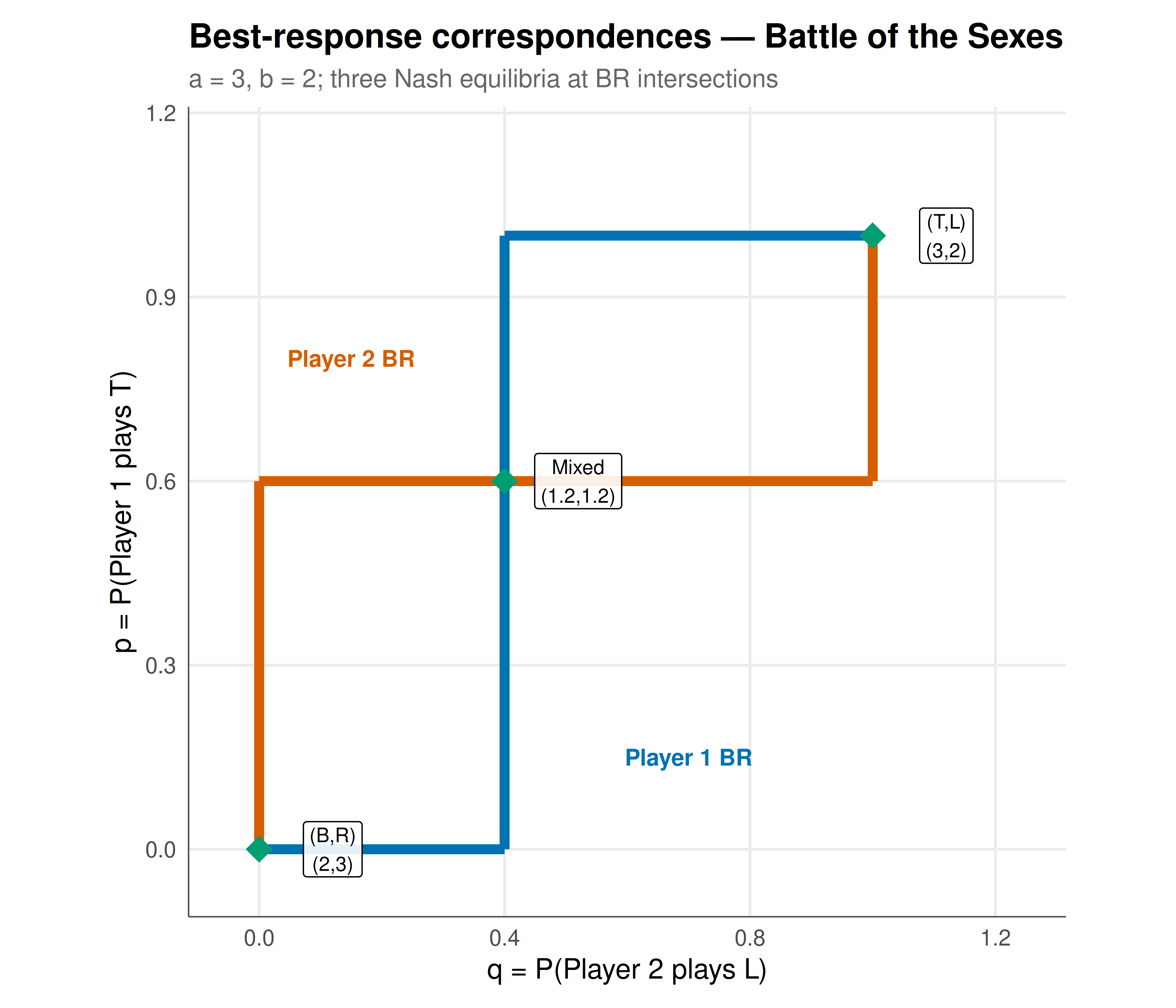
#| fig-cap: "Figure 1. Best-response correspondences for Battle of the Sexes (a=3, b=2). Blue: Player 1's BR (step function in p as a function of q). Red: Player 2's BR (step function in q as a function of p). Green diamonds: Nash equilibria. The two corner intersections are the pure NE; the interior intersection is the mixed NE. The mixed NE is Pareto-dominated by both pure NE. Okabe-Ito palette."
#| dev: [png, pdf]
#| fig-width: 7
#| fig-height: 6
#| dpi: 300
a <- 3; b <- 2
q_indiff <- b / (a + b)  # 2/5: Row indifferent
p_indiff <- a / (a + b)  # 3/5: Col indifferent

eq_points <- tibble(
  q = c(1, 0, q_indiff),
  p = c(1, 0, p_indiff),
  label = c("(T,L)\n(3,2)", "(B,R)\n(2,3)",
            sprintf("Mixed\n(%.1f,%.1f)", a*b/(a+b), a*b/(a+b)))
)

p_br <- ggplot() +
  # Player 1 BR: T if q > q_indiff, B if q < q_indiff
  geom_segment(aes(x = 0, xend = q_indiff, y = 0, yend = 0),
               color = okabe_ito[5], linewidth = 2) +
  geom_segment(aes(x = q_indiff, xend = q_indiff, y = 0, yend = 1),
               color = okabe_ito[5], linewidth = 2) +
  geom_segment(aes(x = q_indiff, xend = 1, y = 1, yend = 1),
               color = okabe_ito[5], linewidth = 2) +
  # Player 2 BR: L if p > p_indiff, R if p < p_indiff
  geom_segment(aes(x = 0, xend = 0, y = 0, yend = p_indiff),
               color = okabe_ito[6], linewidth = 2) +
  geom_segment(aes(x = 0, xend = 1, y = p_indiff, yend = p_indiff),
               color = okabe_ito[6], linewidth = 2) +
  geom_segment(aes(x = 1, xend = 1, y = p_indiff, yend = 1),
               color = okabe_ito[6], linewidth = 2) +
  # Equilibria
  geom_point(data = eq_points, aes(x = q, y = p), color = okabe_ito[3],
             size = 5, shape = 18) +
  geom_label(data = eq_points, aes(x = q, y = p, label = label),
             nudge_x = 0.12, size = 3, fill = "white", alpha = 0.9) +
  annotate("text", x = 0.7, y = 0.15, label = "Player 1 BR",
           color = okabe_ito[5], fontface = "bold", size = 3.5) +
  annotate("text", x = 0.15, y = 0.8, label = "Player 2 BR",
           color = okabe_ito[6], fontface = "bold", size = 3.5) +
  labs(
    title = "Best-response correspondences — Battle of the Sexes",
    subtitle = "a = 3, b = 2; three Nash equilibria at BR intersections",
    x = "q = P(Player 2 plays L)", y = "p = P(Player 1 plays T)"
  ) +
  coord_fixed(xlim = c(-0.05, 1.25), ylim = c(-0.05, 1.15)) +
  theme_publication()

p_br
```
## Interactive figure
```{r}
#| label: fig-bos-payoff-interactive
# Expected payoffs as function of mixing probabilities
grid <- expand.grid(p = seq(0, 1, 0.02), q = seq(0, 1, 0.02))
grid$eu1 <- with(grid, p * q * 3 + (1-p) * (1-q) * 2)
grid$eu2 <- with(grid, p * q * 2 + (1-p) * (1-q) * 3)
grid$total <- grid$eu1 + grid$eu2
grid$text <- with(grid, paste0("p=", round(p,2), " q=", round(q,2),
                                "\nP1: ", round(eu1,2), " P2: ", round(eu2,2),
                                "\nTotal: ", round(total,2)))

p_surface <- ggplot(grid, aes(x = q, y = p, fill = total, text = text)) +
  geom_tile() +
  scale_fill_gradient2(low = okabe_ito[6], mid = okabe_ito[4], high = okabe_ito[3],
                        midpoint = 3, name = "Total payoff") +
  geom_point(data = eq_points, aes(x = q, y = p, fill = NULL, text = label),
             shape = 4, size = 3, stroke = 1.5, color = "black") +
  labs(
    title = "Total welfare across mixing probabilities",
    subtitle = "Coordination (corners) yields higher total payoff than mixed NE (centre)",
    x = "q = P(P2 plays L)", y = "p = P(P1 plays T)"
  ) +
  theme_publication() +
  theme(panel.grid = element_blank())

ggplotly(p_surface, tooltip = "text") |>
  config(displaylogo = FALSE,
         modeBarButtonsToRemove = c("select2d", "lasso2d"))
```
## Interpretation
The Battle of the Sexes reveals a fundamentally different problem from the Prisoner's Dilemma. Where the PD has a unique (inefficient) equilibrium, the BoS has multiple equilibria with no clear way to choose among them. The mixed NE is particularly striking: by randomising, both players earn 1.2 — worse than either pure equilibrium (which gives at least 2 to the less-favoured player). This occurs because randomisation creates a positive probability of miscoordination (52% in the standard parameterization), where both players end up at different events and earn 0. The mixed NE is thus Pareto-dominated by both pure NE, making it an unlikely prediction for real behaviour. The welfare surface visualization confirms this: total surplus is maximised at the coordination corners and minimised along the miscoordination diagonal. This analysis motivates several important extensions in game theory: Thomas Schelling's concept of **focal points** (conventions or salient features that allow players to coordinate without communication), Aumann's **correlated equilibrium** (a mediator who sends private recommendations, potentially achieving better outcomes than any Nash equilibrium), and pre-play communication (cheap talk, which can help in BoS but not in the PD). In practice, BoS dynamics govern technology adoption, where competing standards must converge, and international policy coordination, where countries prefer alignment but disagree on the terms.
## Extensions & related tutorials
- [Mixed-strategy Nash equilibrium](../../foundations/nash-equilibrium-mixed/) — computing the mixed NE for general 2×2 games.
- [Stag Hunt](../stag-hunt/) — a coordination game without conflicting preferences.
- [Chicken / Hawk-Dove](../chicken-hawk-dove/) — an anti-coordination game.
- [Correlated equilibrium](../../foundations/correlated-equilibrium/) — going beyond Nash with a mediator.
- [2×2 Nash Explorer (Shiny)](../../../shiny/tutorials/two-by-two-nash-explorer-tutorial/) — interactive exploration of BoS parameters.
## References
::: {#refs}
:::