---
title: "Building the 2×2 Nash Equilibrium Explorer — a Shiny tutorial"
description: "Step-by-step tutorial for building an interactive Shiny app that computes and visualizes Nash equilibria for arbitrary 2×2 bimatrix games, with best-response plots and expected payoff surfaces."
author: "Raban Heller"
date: 2026-05-08
date-modified: 2026-05-08
categories:
- shiny-tutorial
- nash-equilibrium
- interactive
- bimatrix-games
keywords: ["Shiny", "Nash equilibrium", "2x2 game", "best response", "interactive", "bimatrix"]
labels: ["shiny-app", "foundational-tool"]
tier: 1
bibliography: ../../../references.bib
vgwort: "TODO_VGWORT_shiny_two-by-two-nash-explorer-tutorial"
image: thumbnail.png
image-alt: "Screenshot of the 2×2 Nash Equilibrium Explorer Shiny app"
citation:
type: webpage
url: https://r-heller.github.io/equilibria/shiny/tutorials/two-by-two-nash-explorer-tutorial/
license: "CC BY-SA 4.0"
draft: false
has_static_fig: true
has_interactive_fig: true
has_shiny_app: "two-by-two-nash-explorer"
---
```{r}
#| label: setup
#| include: false
library(ggplot2)
library(dplyr)
library(plotly)
okabe_ito <- c("#E69F00", "#56B4E9", "#009E73", "#F0E442",
"#0072B2", "#D55E00", "#CC79A7", "#999999")
theme_publication <- function(base_size = 12) {
theme_minimal(base_size = base_size) +
theme(
plot.title = element_text(size = base_size * 1.2, face = "bold"),
plot.subtitle = element_text(size = base_size * 0.9, color = "grey40"),
axis.line = element_line(color = "grey30", linewidth = 0.3),
panel.grid.minor = element_blank(),
legend.position = "bottom",
plot.margin = margin(10, 10, 10, 10)
)
}
```
## Introduction & motivation
The 2×2 bimatrix game is the simplest non-trivial strategic interaction: two players, each with two strategies, producing a 2×2 payoff matrix for each player. Despite its simplicity, the 2×2 game encompasses the Prisoner's Dilemma, Battle of the Sexes, Matching Pennies, Stag Hunt, Chicken, and many other canonical games. Computing Nash equilibria for 2×2 games requires checking pure-strategy profiles for mutual best responses and solving a pair of linear indifference equations for mixed equilibria — straightforward mathematics, but tedious to do by hand and hard to visualize. The **2×2 Nash Equilibrium Explorer** is a Shiny app that lets users enter arbitrary payoff matrices, instantly see all Nash equilibria (pure and mixed), and explore best-response correspondences and expected payoff surfaces interactively. This tutorial walks through the app's construction step by step: the equilibrium solver, the reactive UI, the best-response visualization, and the payoff surface plots. Building this app is an exercise in combining game-theoretic computation with interactive web technology — a pattern that recurs throughout this site's Shiny applications.
## The Nash equilibrium solver
The core algorithm checks all four pure-strategy profiles and then solves for the mixed equilibrium.
```{r}
#| label: solver
solve_nash_2x2 <- function(A, B) {
  equilibria <- list()

  # Pure strategy NE: check all four profiles
  for (i in 1:2) {
    for (j in 1:2) {
      # Is i a best response for Row given Col plays j?
      br_row <- (A[i, j] >= A[3 - i, j])
      # Is j a best response for Col given Row plays i?
      br_col <- (B[i, j] >= B[i, 3 - j])

      if (br_row && br_col) {
        equilibria <- c(equilibria, list(list(
          type = "Pure",
          p = ifelse(i == 1, 1, 0),  # P(Row plays Top)
          q = ifelse(j == 1, 1, 0),  # P(Col plays Left)
          row_payoff = A[i, j],
          col_payoff = B[i, j]
        )))
      }
    }
  }

  # Mixed strategy NE
  # Row indifference: q*A[1,1] + (1-q)*A[1,2] = q*A[2,1] + (1-q)*A[2,2]
  denom_q <- (A[1,1] - A[2,1]) - (A[1,2] - A[2,2])
  # Col indifference: p*B[1,1] + (1-p)*B[2,1] = p*B[1,2] + (1-p)*B[2,2]
  denom_p <- (B[1,1] - B[2,1]) - (B[1,2] - B[2,2])

  if (abs(denom_q) > 1e-10 && abs(denom_p) > 1e-10) {
    q_star <- (A[2,2] - A[1,2]) / denom_q
    p_star <- (B[2,2] - B[2,1]) / denom_p

    if (p_star > 0 && p_star < 1 && q_star > 0 && q_star < 1) {
      row_payoff <- p_star * (q_star * A[1,1] + (1 - q_star) * A[1,2]) +
                    (1 - p_star) * (q_star * A[2,1] + (1 - q_star) * A[2,2])
      col_payoff <- p_star * (q_star * B[1,1] + (1 - q_star) * B[1,2]) +
                    (1 - p_star) * (q_star * B[2,1] + (1 - q_star) * B[2,2])

      equilibria <- c(equilibria, list(list(
        type = "Mixed",
        p = round(p_star, 4),
        q = round(q_star, 4),
        row_payoff = round(row_payoff, 4),
        col_payoff = round(col_payoff, 4)
      )))
    }
  }

  equilibria
}

# --- Test with classic games ---
cat("=== Prisoner's Dilemma ===\n")
A_pd <- matrix(c(3, 5, 0, 1), nrow = 2)
B_pd <- matrix(c(3, 0, 5, 1), nrow = 2)
pd_eq <- solve_nash_2x2(A_pd, B_pd)
for (eq in pd_eq) cat(sprintf("  %s NE: p=%.2f, q=%.2f, payoffs=(%.2f, %.2f)\n",
                                eq$type, eq$p, eq$q, eq$row_payoff, eq$col_payoff))
cat("\n=== Battle of the Sexes ===\n")
A_bos <- matrix(c(3, 0, 0, 2), nrow = 2)
B_bos <- matrix(c(2, 0, 0, 3), nrow = 2)
bos_eq <- solve_nash_2x2(A_bos, B_bos)
for (eq in bos_eq) cat(sprintf("  %s NE: p=%.2f, q=%.2f, payoffs=(%.2f, %.2f)\n",
                                eq$type, eq$p, eq$q, eq$row_payoff, eq$col_payoff))
cat("\n=== Matching Pennies ===\n")
A_mp <- matrix(c(1, -1, -1, 1), nrow = 2)
B_mp <- matrix(c(-1, 1, 1, -1), nrow = 2)
mp_eq <- solve_nash_2x2(A_mp, B_mp)
for (eq in mp_eq) cat(sprintf("  %s NE: p=%.2f, q=%.2f, payoffs=(%.2f, %.2f)\n",
                                eq$type, eq$p, eq$q, eq$row_payoff, eq$col_payoff))
```
## Best response visualization
```{r}
#| label: fig-br-static
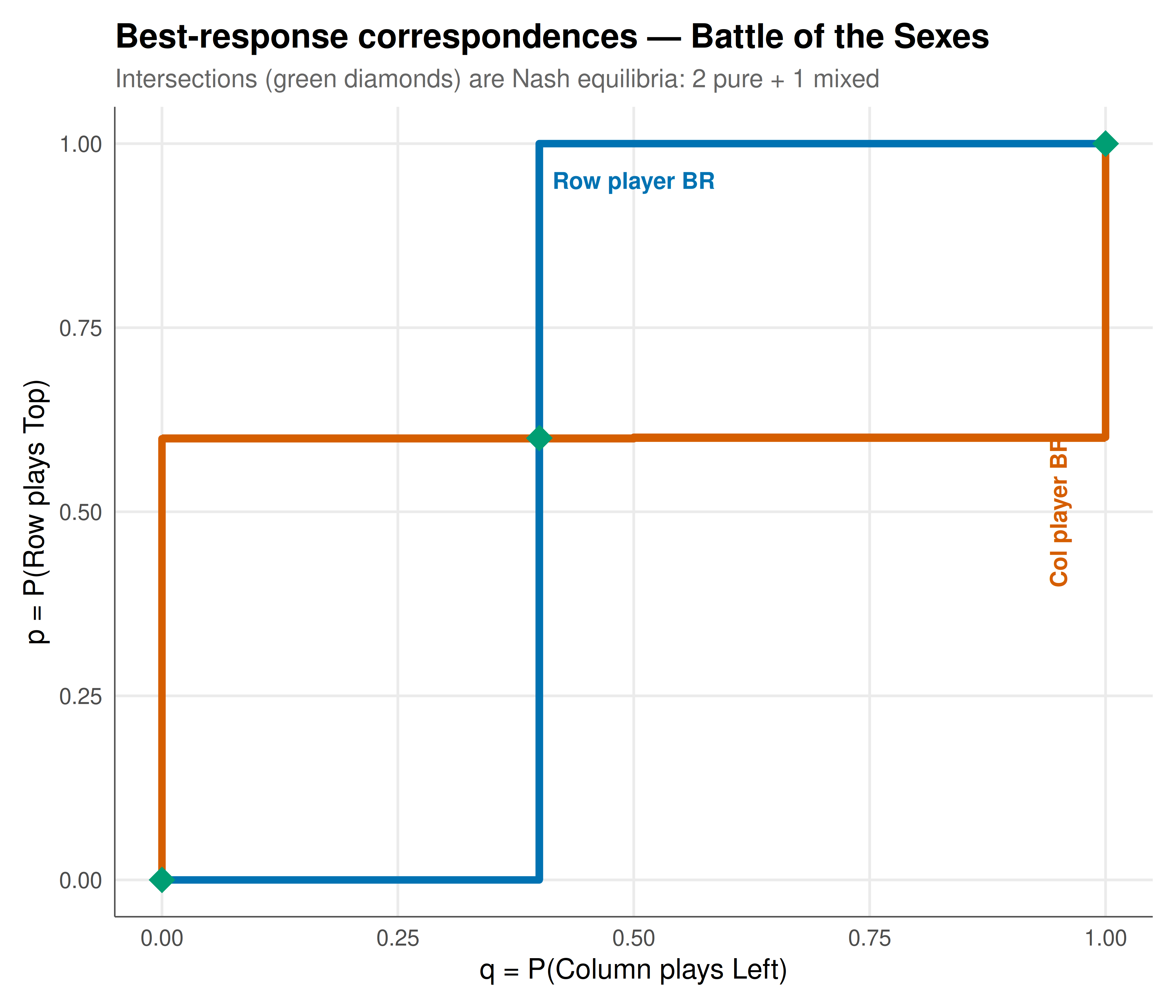
#| fig-cap: "Figure 1. Best-response correspondences for Battle of the Sexes. Blue step function: Row player's BR as a function of q (Col's mixing probability). Red step function: Col's BR as a function of p. Green diamonds mark Nash equilibria — two pure (corners) and one mixed (interior). The best-response plot is the core visual output of the Shiny app. Okabe-Ito palette."
#| dev: [png, pdf]
#| fig-width: 7
#| fig-height: 6
#| dpi: 300
A <- A_bos; B <- B_bos

# Row player BR
q_seq <- seq(0, 1, length.out = 500)
row_br <- sapply(q_seq, function(q) {
  coeff <- q * (A[1,1] - A[2,1]) + (1 - q) * (A[1,2] - A[2,2])
  if (abs(coeff) < 1e-10) return(NA)
  if (coeff > 0) return(1) else return(0)
})

# Column player BR
p_seq <- seq(0, 1, length.out = 500)
col_br <- sapply(p_seq, function(p) {
  coeff <- p * (B[1,1] - B[1,2]) + (1 - p) * (B[2,1] - B[2,2])
  if (abs(coeff) < 1e-10) return(NA)
  if (coeff > 0) return(1) else return(0)
})

row_br_df <- tibble(q = q_seq, p_br = row_br) |> filter(!is.na(p_br))
col_br_df <- tibble(p = p_seq, q_br = col_br) |> filter(!is.na(q_br))

# Add vertical segments for BRs at indifference points
q_indiff <- (A[2,2] - A[1,2]) / ((A[1,1] - A[2,1]) - (A[1,2] - A[2,2]))
p_indiff <- (B[2,2] - B[2,1]) / ((B[1,1] - B[2,1]) - (B[1,2] - B[2,2]))

eq_points <- do.call(rbind, lapply(bos_eq, function(e) {
  data.frame(q = e$q, p = e$p, label = paste0(e$type, ": (", e$p, ", ", e$q, ")"))
}))

ggplot() +
  # Row BR (blue)
  geom_step(data = row_br_df, aes(x = q, y = p_br), color = okabe_ito[5],
            linewidth = 1.5, direction = "mid") +
  geom_segment(aes(x = q_indiff, xend = q_indiff, y = 0, yend = 1),
               color = okabe_ito[5], linewidth = 1.5) +
  # Col BR (red)
  geom_step(data = col_br_df, aes(x = q_br, y = p), color = okabe_ito[6],
            linewidth = 1.5, direction = "mid") +
  geom_segment(aes(x = 0, xend = 1, y = p_indiff, yend = p_indiff),
               color = okabe_ito[6], linewidth = 1.5) +
  # Equilibrium points
  geom_point(data = eq_points, aes(x = q, y = p), color = okabe_ito[3],
             size = 5, shape = 18) +
  annotate("text", x = 0.5, y = 0.95, label = "Row player BR", color = okabe_ito[5],
           size = 3.5, fontface = "bold") +
  annotate("text", x = 0.95, y = 0.5, label = "Col player BR", color = okabe_ito[6],
           size = 3.5, fontface = "bold", angle = 90) +
  labs(
    title = "Best-response correspondences — Battle of the Sexes",
    subtitle = "Intersections (green diamonds) are Nash equilibria: 2 pure + 1 mixed",
    x = "q = P(Column plays Left)", y = "p = P(Row plays Top)"
  ) +
  theme_publication()
```
## Interactive expected payoff surface
```{r}
#| label: fig-payoff-surface-interactive
A <- A_bos; B <- B_bos

grid <- expand.grid(p = seq(0, 1, by = 0.02), q = seq(0, 1, by = 0.02))
grid$row_payoff <- with(grid,
  p * (q * A[1,1] + (1-q) * A[1,2]) + (1-p) * (q * A[2,1] + (1-q) * A[2,2])
)
grid$col_payoff <- with(grid,
  p * (q * B[1,1] + (1-q) * B[1,2]) + (1-p) * (q * B[2,1] + (1-q) * B[2,2])
)

grid_text <- grid |>
  mutate(text = paste0("p=", round(p, 2), " q=", round(q, 2),
                       "\nRow payoff: ", round(row_payoff, 2),
                       "\nCol payoff: ", round(col_payoff, 2)))

p_surface <- ggplot(grid_text, aes(x = q, y = p, fill = row_payoff, text = text)) +
  geom_tile() +
  scale_fill_gradient2(low = okabe_ito[6], mid = okabe_ito[4], high = okabe_ito[3],
                        midpoint = mean(grid$row_payoff), name = "Row payoff") +
  # Mark equilibria
  geom_point(data = eq_points, aes(x = q, y = p, fill = NULL, text = label),
             color = "black", size = 3, shape = 4, stroke = 1.5) +
  labs(
    title = "Row player expected payoff — Battle of the Sexes",
    x = "q = P(Col plays Left)", y = "p = P(Row plays Top)"
  ) +
  theme_publication() +
  theme(panel.grid = element_blank())

ggplotly(p_surface, tooltip = "text") |>
  config(displaylogo = FALSE,
         modeBarButtonsToRemove = c("select2d", "lasso2d"))
```
## Shiny app architecture
The complete app (`shiny-apps/01-two-by-two-nash-explorer/app.R`) has four main components:
1. **Payoff input panel**: Eight `numericInput` fields arranged as a 2×2 bimatrix table, plus a `selectInput` for preset games (PD, BoS, Matching Pennies, Stag Hunt, Chicken).
2. **Nash solver** (`solve_nash_2x2`): The same function shown above, wrapped in a `reactive()` expression that recomputes whenever any payoff input changes.
3. **Best-response plot**: A `plotlyOutput` rendering the step-function best-response correspondences for both players, with equilibrium points marked.
4. **Expected payoff contour plots**: Two side-by-side `plotlyOutput` panels showing the expected payoff surface for each player as a function of the mixing probabilities $(p, q)$.
The app is fully self-contained — no external data dependencies — and can be deployed to shinyapps.io or run locally with `shiny::runApp("shiny-apps/01-two-by-two-nash-explorer/")`.
## Interpretation
The 2×2 Nash Explorer makes visible the geometry of strategic interaction. The best-response plot reveals why different game structures produce different equilibrium configurations: in the Prisoner's Dilemma, both BRs point to (Defect, Defect) regardless of the opponent's mix — the unique NE is a dominant-strategy equilibrium. In Battle of the Sexes, the BRs create an S-shaped intersection pattern producing two pure NE at the corners and one mixed NE in the interior. In Matching Pennies, the BRs are step functions that cross only at the centre — the unique NE is completely mixed at (1/2, 1/2). The expected payoff surfaces show that at a mixed NE, neither player can unilaterally improve their expected payoff — the mixed NE sits at a saddle point of the individual payoff landscapes, not a maximum. This geometric insight — that mixed NE are not outcomes players actively seek but rather fixed points of the best-response dynamics — is fundamental to interpreting mixed equilibria correctly and connects to @nash_1950's original existence proof via Kakutani's fixed-point theorem.
## Extensions & related tutorials
- [Mixed-strategy Nash equilibrium in 2×2 games](../../../tutorials/foundations/nash-equilibrium-mixed/) — the mathematical foundations behind this app.
- [Replicator dynamics for RPS](../../../tutorials/evolutionary-gt/replicator-dynamics-rps/) — extending to 3-strategy dynamics.
- [Shiny app: Replicator dynamics explorer](../replicator-dynamics-rps-simplex-tutorial/) — interactive simplex visualization.
- [Publication-ready ggplot2 theme](../../../tutorials/visualization-and-communication/publication-ready-ggplot-theme/) — the theme used in this app.
- [The iterated Prisoner's Dilemma](../../../tutorials/classical-games/iterated-prisoners-dilemma-axelrod/) — extending to repeated interactions.
## References
::: {#refs}
:::