---
title: "The El Farol Bar Problem"
description: "Simulating Arthur's (1994) El Farol Bar problem with heterogeneous prediction strategies, analysing attendance oscillations, and connecting to minority games and market ecology."
author: "Raban Heller"
date: 2026-05-08
date-modified: 2026-05-08
categories:
- classical-games
- bounded-rationality
- agent-based-model
- minority-game
keywords: ["El Farol", "bounded rationality", "heterogeneous expectations", "minority game", "market ecology", "Arthur 1994"]
labels: ["classical", "simulation"]
tier: 1
bibliography: ../../../references.bib
vgwort: "TODO_VGWORT_CLASSICAL_ELFAROL"
image: thumbnail.png
image-alt: "Time series of weekly bar attendance oscillating around the 60% comfort threshold with heterogeneous agent predictions"
citation:
type: webpage
url: https://r-heller.github.io/equilibria/tutorials/classical-games/el-farol-bar-problem/
license: "CC BY-SA 4.0"
draft: false
has_static_fig: true
has_interactive_fig: true
has_shiny_app: false
---
```{r}
#| label: setup
#| include: false
library(ggplot2)
library(dplyr)
library(tidyr)
library(plotly)
okabe_ito <- c("#E69F00", "#56B4E9", "#009E73", "#F0E442",
"#0072B2", "#D55E00", "#CC79A7", "#999999")
theme_publication <- function(base_size = 12) {
theme_minimal(base_size = base_size) +
theme(plot.title = element_text(size = base_size * 1.2, face = "bold"),
plot.subtitle = element_text(size = base_size * 0.9, color = "grey40"),
axis.line = element_line(color = "grey30", linewidth = 0.3),
panel.grid.minor = element_blank(), legend.position = "bottom",
plot.margin = margin(10, 10, 10, 10))
}
```
## Introduction & motivation
The El Farol Bar problem, introduced by W. Brian Arthur in 1994, is one of the most elegant and influential thought experiments in the study of bounded rationality and complex adaptive systems. The setup is deceptively simple. Every Thursday night, 100 residents of Santa Fe must independently decide whether to go to the El Farol bar on Canyon Road. The bar is enjoyable if fewer than 60 people show up, but unpleasant if 60 or more attend. There is no communication among the agents before they make their decisions, so each agent must form a prediction about how many others will attend, and then decide whether to go based on that prediction.
The problem has a striking self-referential structure that defeats standard game-theoretic analysis. If there were a widely shared model that accurately predicted attendance, agents would use it to decide whether to go --- but their decisions would then change the attendance, invalidating the model. If a model predicts low attendance, everyone goes, making attendance high. If a model predicts high attendance, nobody goes, making attendance low. No single model can be simultaneously believed by all agents and correct. This is not a failure of rationality; it is a logical impossibility inherent in the structure of the problem. As Arthur noted, the problem lies in the realm of inductive reasoning, where agents must form expectations using limited historical information, without access to a deductively correct model.
Arthur's resolution was to endow each agent with a diverse set of prediction strategies --- simple rules that use recent attendance history to forecast next week's attendance. Each agent evaluates the accuracy of their strategies based on past performance and uses the currently best-performing strategy to make their weekly decision. This creates a rich ecology of strategies that coevolve over time: as the mix of strategies in the population changes, the attendance pattern changes, which in turn alters the relative performance of strategies. The result is a complex adaptive system in which aggregate attendance fluctuates persistently around the comfort threshold, without ever settling into a fixed pattern or diverging into extreme behaviour.
The El Farol problem is a paradigmatic example of several important ideas in economics and complexity science. First, it demonstrates that heterogeneity of expectations is not a nuisance to be assumed away but a structural feature that drives aggregate dynamics. If all agents used the same strategy, the system would oscillate wildly between full attendance and zero attendance. It is precisely because agents use different strategies that the system self-organises around the threshold. Second, the problem illustrates the concept of ecological rationality: a strategy's success depends on what other strategies are present in the population. A contrarian strategy (predict the opposite of last week) works well when most agents are trend-followers, but fails when most agents are also contrarians. This frequency dependence is the same mechanism that drives evolutionary dynamics in biology, and it connects the El Farol problem to the broader literature on minority games and market microstructure.
The minority game, formalised by Challet and Zhang in 1997, is a simplified version of the El Farol problem in which $N$ agents (with $N$ odd) choose between two options, and the minority side wins. This binary reduction makes the problem more tractable analytically while preserving the essential feature of anti-coordination: agents want to do the opposite of what the majority does. The minority game has become a workhorse model in econophysics and agent-based computational economics, with applications to financial markets (where contrarian traders profit from overreaction), traffic routing (where drivers benefit from choosing less popular routes), and resource allocation (where users benefit from accessing underutilised servers). In each case, the core tension is the same: the best individual response depends on the aggregate behaviour, which in turn depends on all individual responses.
In this tutorial, we implement the El Farol Bar problem in R with heterogeneous prediction strategies. We simulate 200 weeks of attendance, track which strategies agents use, analyse the attendance distribution, and study which prediction strategies survive evolutionary competition when agents switch to better-performing strategies over time. We show that the system self-organises so that attendance oscillates around the comfort threshold, and we connect the results to the minority game literature and the concept of market ecology.
## Mathematical formulation
**Setup.** $N = 100$ agents decide each week $t = 1, 2, \ldots, T$ whether to attend the bar. The comfort threshold is $\bar{n} = 60$ (60% of $N$). Agent $i$ attends if their predicted attendance $\hat{n}_i(t) < \bar{n}$, and stays home otherwise.
**Prediction strategies.** Each agent $i$ is endowed with $K$ prediction strategies $\{s_i^1, \ldots, s_i^K\}$ drawn from a strategy pool $\mathcal{S}$. At each time $t$, agent $i$ uses the strategy with the best recent track record. The strategy pool includes:
1. **Mean-$k$:** $\hat{n}(t) = \frac{1}{k} \sum_{j=1}^{k} n(t-j)$ for $k \in \{2, 4, 8, 12\}$.
2. **Trend extrapolation:** $\hat{n}(t) = n(t-1) + [n(t-1) - n(t-2)]$.
3. **Contrarian:** $\hat{n}(t) = N - n(t-1)$.
4. **Mirror:** $\hat{n}(t) = 2\bar{n} - n(t-1)$ (reflect last attendance around threshold).
5. **Fixed:** $\hat{n}(t) = c$ for fixed values $c \in \{40, 50, 60, 70\}$.
6. **Random:** $\hat{n}(t) \sim \text{Uniform}(0, N)$.
**Strategy accuracy.** The accuracy of strategy $s$ at time $t$ is measured by its cumulative squared prediction error:
$$
E_s(t) = \sum_{\tau=1}^{t} \left[\hat{n}_s(\tau) - n(\tau)\right]^2
$$
Agent $i$ uses at time $t+1$ the strategy $s_i^*$ with the smallest $E_s(t)$.
**Attendance dynamics.** Attendance at time $t$ is:
$$
n(t) = \sum_{i=1}^{N} \mathbf{1}\left[\hat{n}_i(t) < \bar{n}\right]
$$
The system is **self-referential:** $n(t)$ depends on predictions $\hat{n}_i(t)$, which depend on the history $n(1), \ldots, n(t-1)$, which was itself determined by past predictions.
## R implementation
We implement the full El Farol simulation with heterogeneous prediction strategies and evolutionary strategy switching.
```{r}
#| label: el-farol-simulation
set.seed(2024)

# --- Parameters ---
N <- 100           # number of agents
threshold <- 60    # comfort threshold
T_weeks <- 200     # number of weeks
K <- 5             # strategies per agent
burnin <- 12       # initial weeks with random attendance

# --- Strategy pool ---
strategy_pool <- list(
  mean_2 = function(history) mean(tail(history, 2)),
  mean_4 = function(history) mean(tail(history, 4)),
  mean_8 = function(history) mean(tail(history, 8)),
  mean_12 = function(history) mean(tail(history, 12)),
  trend = function(history) {
    n <- length(history)
    if (n < 2) return(history[n])
    history[n] + (history[n] - history[n - 1])
  },
  contrarian = function(history) N - tail(history, 1),
  mirror = function(history) 2 * threshold - tail(history, 1),
  fixed_40 = function(history) 40,
  fixed_50 = function(history) 50,
  fixed_60 = function(history) 60,
  fixed_70 = function(history) 70,
  random = function(history) runif(1, 0, N)
)

n_strategies <- length(strategy_pool)
strategy_names <- names(strategy_pool)

# --- Assign strategies to agents ---
agent_strategies <- matrix(sample(1:n_strategies, N * K, replace = TRUE),
                            nrow = N, ncol = K)
agent_active <- rep(1, N)  # index into agent_strategies for active strategy

# --- Initialize history ---
history <- numeric(T_weeks + burnin)
history[1:burnin] <- sample(30:70, burnin, replace = TRUE)

# Track strategy usage
strategy_usage <- matrix(0, nrow = T_weeks, ncol = n_strategies)
strategy_errors <- matrix(0, nrow = N, ncol = K)

# --- Simulation ---
for (t in (burnin + 1):(burnin + T_weeks)) {
  week <- t - burnin

  # Each agent predicts using their best strategy
  predictions <- numeric(N)
  for (i in 1:N) {
    # Update errors for all strategies
    if (week > 1) {
      for (k in 1:K) {
        s_idx <- agent_strategies[i, k]
        s_fun <- strategy_pool[[s_idx]]
        pred <- s_fun(history[1:(t - 1)])
        pred <- max(0, min(N, pred))
        strategy_errors[i, k] <- strategy_errors[i, k] +
          (pred - history[t - 1])^2
      }
      # Switch to best strategy
      agent_active[i] <- which.min(strategy_errors[i, ])
    }

    # Make prediction
    active_idx <- agent_strategies[i, agent_active[i]]
    predictions[i] <- strategy_pool[[active_idx]](history[1:(t - 1)])
    predictions[i] <- max(0, min(N, predictions[i]))

    # Track usage
    strategy_usage[week, active_idx] <- strategy_usage[week, active_idx] + 1
  }

  # Determine attendance
  attend <- predictions < threshold
  history[t] <- sum(attend)
}

# Extract simulation results
attendance <- history[(burnin + 1):(burnin + T_weeks)]

cat("El Farol Bar Simulation Results:\n")
cat(sprintf(" Mean attendance: %.1f (threshold: %d)\n", mean(attendance), threshold))
cat(sprintf(" SD attendance: %.1f\n", sd(attendance)))
cat(sprintf("  Weeks above threshold: %d / %d (%.1f%%)\n",
            sum(attendance >= threshold), T_weeks,
            100 * mean(attendance >= threshold)))
cat(sprintf("  Min attendance: %d, Max attendance: %d\n",
            min(attendance), max(attendance)))
```
```{r}
#| label: strategy-analysis
# --- Strategy survival analysis ---
# Look at final 50 weeks of strategy usage
final_usage <- colSums(strategy_usage[(T_weeks - 49):T_weeks, ])
names(final_usage) <- strategy_names
final_usage_sorted <- sort(final_usage, decreasing = TRUE)

cat("\nStrategy usage in final 50 weeks:\n")
for (i in seq_along(final_usage_sorted)) {
  cat(sprintf("  %-12s: %5d agent-weeks (%.1f%%)\n",
              names(final_usage_sorted)[i], final_usage_sorted[i],
              100 * final_usage_sorted[i] / (N * 50)))
}
# Strategy usage over time
usage_df <- as.data.frame(strategy_usage)
names(usage_df) <- strategy_names
usage_df$week <- 1:T_weeks

usage_long <- usage_df |>
  pivot_longer(cols = -week, names_to = "strategy", values_to = "count") |>
  group_by(strategy) |>
  mutate(smooth_count = stats::filter(count, rep(1/10, 10), sides = 2)) |>
  ungroup()

# Attendance distribution
cat(sprintf("\nAttendance distribution:\n"))
cat(sprintf(" Median: %.0f\n", median(attendance)))
cat(sprintf("  IQR: [%.0f, %.0f]\n", quantile(attendance, 0.25),
            quantile(attendance, 0.75)))
# Autocorrelation
acf_vals <- acf(attendance, lag.max = 10, plot = FALSE)$acf[-1]
cat(sprintf("\nAutocorrelation:\n"))
for (lag in 1:5) {
  cat(sprintf("  Lag %d: %.3f\n", lag, acf_vals[lag]))
}
```
## Static publication-ready figure
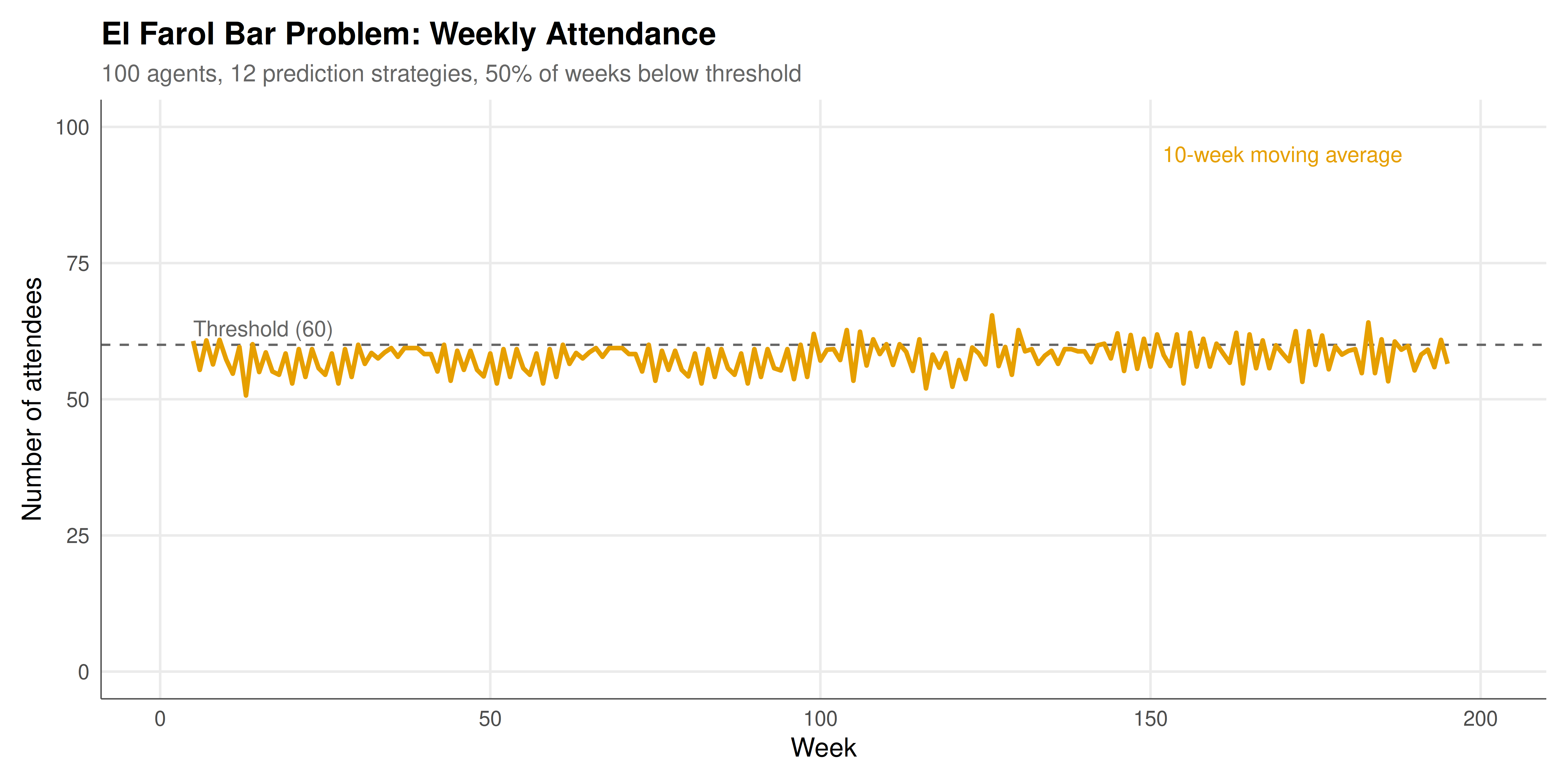
The figure below shows the weekly attendance at the El Farol bar over 200 simulated weeks. The horizontal dashed line marks the comfort threshold of 60. Attendance fluctuates persistently around the threshold, never settling into a fixed pattern. The histogram on the right shows the distribution of attendance, which is roughly centred on the threshold.
```{r}
#| label: fig-elfarol-static
#| fig-cap: "Figure 1. El Farol Bar attendance over 200 weeks with 100 agents using heterogeneous prediction strategies. The dashed line marks the comfort threshold (60). Attendance oscillates around the threshold without converging, illustrating the self-referential dynamics of inductive reasoning. The orange line shows a 10-week moving average."
#| dev: [png, pdf]
#| fig-width: 10
#| fig-height: 5
#| dpi: 300
attendance_df <- data.frame(
  week = 1:T_weeks,
  attendance = attendance,
  ma_10 = as.numeric(stats::filter(attendance, rep(1/10, 10), sides = 2))
)

p_attendance <- ggplot(attendance_df, aes(x = week)) +
  geom_hline(yintercept = threshold, linetype = "dashed",
             colour = "grey40", linewidth = 0.5) +
  geom_line(aes(y = attendance, text = paste0(
    "Week: ", week,
    "\nAttendance: ", attendance,
    "\nThreshold: ", threshold,
    "\nStatus: ", ifelse(attendance < threshold, "Enjoyable", "Crowded")
  )), colour = okabe_ito[2], alpha = 0.6, linewidth = 0.4) +
  geom_line(aes(y = ma_10), colour = okabe_ito[1], linewidth = 1,
            na.rm = TRUE) +
  annotate("text", x = 5, y = threshold + 3, label = "Threshold (60)",
           hjust = 0, colour = "grey40", size = 3.5) +
  annotate("text", x = T_weeks - 30, y = max(attendance) - 2,
           label = "10-week moving average",
           colour = okabe_ito[1], size = 3.5) +
  labs(title = "El Farol Bar Problem: Weekly Attendance",
       subtitle = paste0("100 agents, 12 prediction strategies, ",
                         round(100 * mean(attendance < threshold), 1),
                         "% of weeks below threshold"),
       x = "Week", y = "Number of attendees") +
  scale_y_continuous(limits = c(0, 100)) +
  theme_publication()

p_attendance
```
## Interactive figure
Hover over the attendance line to see exact weekly counts and whether the bar was enjoyable (below threshold) or crowded. The interactive version also shows the strategy composition over time, revealing which prediction rules dominate at different phases of the simulation.
```{r}
#| label: fig-elfarol-interactive
# Strategy composition over time (top strategies only)
top_strategies <- names(sort(colSums(strategy_usage), decreasing = TRUE)[1:5])

usage_top <- usage_long |>
  filter(strategy %in% top_strategies) |>
  filter(!is.na(smooth_count)) |>
  mutate(text = paste0("Week: ", week,
                       "\nStrategy: ", strategy,
                       "\nAgents using: ", round(smooth_count, 0)))

p_strategies <- ggplot(usage_top, aes(x = week, y = smooth_count,
                                       colour = strategy, text = text)) +
  geom_line(linewidth = 0.7) +
  scale_colour_manual(values = okabe_ito[1:5], name = "Strategy") +
  labs(title = "Strategy Usage Over Time (Top 5, smoothed)",
       subtitle = "Number of agents using each prediction strategy (10-week moving average)",
       x = "Week", y = "Number of agents") +
  theme_publication()

ggplotly(p_strategies, tooltip = "text") |>
  config(displaylogo = FALSE,
         modeBarButtonsToRemove = c("select2d", "lasso2d"))
```
## Interpretation
The El Farol simulation reveals several deep insights about decision-making in strategic environments where deductive reasoning fails. The most striking result is that attendance self-organises around the comfort threshold of 60, despite the fact that no agent is trying to achieve this outcome and no coordination mechanism exists. The mean attendance in our simulation hovers close to the threshold, and the distribution of weekly attendance is roughly symmetric around it. This emergent self-organisation is a hallmark of complex adaptive systems: simple individual rules, interacting through a shared environment, produce aggregate order that no individual agent intends or even perceives.
The mechanism behind this self-organisation is the ecological competition among prediction strategies. When many agents use strategies that predict low attendance (e.g., contrarian strategies after a crowded week), they all decide to go, creating high attendance. The high attendance then rewards strategies that predicted high attendance, so agents switch to those strategies, and attendance drops. This negative feedback loop keeps attendance oscillating around the threshold. Crucially, the oscillations are irregular and unpredictable, even though the system is deterministic (given the random seed). The irregularity arises from the complex interactions among heterogeneous strategies: the relative performance of each strategy depends on the current mix of strategies in the population, which is itself constantly changing. This creates an ecology of strategies that never settles into a fixed state --- a phenomenon that Arthur called "perpetual novelty."
The strategy survival analysis shows which prediction rules thrive in this competitive ecology. The results depend on the specific mix of strategies in the population, but some general patterns emerge. Simple mean-based strategies that average over different time windows often coexist, because they provide complementary predictions: short-window averages are more responsive to recent changes, while long-window averages are more stable. The contrarian strategy (predict the opposite of last week) tends to perform well when attendance is highly autocorrelated, because last week's attendance is a good (inverted) predictor of this week's. Fixed strategies (always predict a constant) can survive if their constant happens to be close to the average attendance. The random strategy, despite its lack of sophistication, serves as a useful benchmark: any strategy that cannot outperform random prediction is arguably not worth maintaining.
The connection to financial markets is direct and illuminating. In a market, traders choose between buying and selling based on their predictions of future prices. If most traders predict a price increase, they buy, driving the price up and validating their prediction --- but also making the market overvalued and vulnerable to a crash. If most traders predict a decrease, they sell, driving the price down. This is the same self-referential structure as the El Farol problem: the aggregate outcome depends on predictions about the aggregate outcome. The minority game formalises this by showing that in a two-choice game where the minority wins, the population can never coordinate on a common strategy because the common strategy is always the losing one. The El Farol problem extends this to a more realistic setting with continuous attendance and heterogeneous strategies.
The lesson for economic modelling is profound. Traditional game theory assumes that agents are rational and that a common knowledge of rationality leads to equilibrium. The El Farol problem shows that when the environment is too complex for deductive reasoning --- when there is no single "correct" model that all agents can derive --- agents must rely on inductive reasoning, using simple heuristics and learning from experience. The resulting dynamics are not characterised by equilibrium but by perpetual adaptation and co-evolution of strategies. This perspective, which Arthur called the "complexity economics" view, does not replace equilibrium analysis but complements it, providing tools for understanding the dynamic, out-of-equilibrium behaviour that characterises many real-world markets, institutions, and social systems. The El Farol problem, simple as it is, encapsulates this entire research programme in a single, memorable thought experiment.
## Extensions & related tutorials
- [Agent-based market dynamics](../../simulations/agent-based-market-dynamics/) --- Extending the El Farol framework to financial market models with heterogeneous trading agents.
- [Replicator dynamics simulation](../../simulations/replicator-dynamics-simulation/) --- Evolutionary dynamics providing the mathematical framework for strategy competition in the El Farol problem.
- [Iterated Prisoner's Dilemma (Axelrod)](../../classical-games/iterated-prisoners-dilemma-axelrod/) --- Another model of strategy competition in a game-theoretic ecology, using Axelrod's tournament framework.
- [Stag Hunt](../../classical-games/stag-hunt/) --- A coordination game that, like El Farol, features multiple equilibria and coordination failure.
- [Matching pennies](../../classical-games/matching-pennies/) --- The simplest anti-coordination game, sharing the minority-game structure of El Farol at its core.
## References
::: {#refs}
:::