---
title: "Rubinstein's alternating-offers bargaining game"
description: "Implement Rubinstein's infinite-horizon alternating-offers model in R, derive the unique subgame-perfect equilibrium as a function of discount factors, and visualise how patience determines bargaining power."
author: "Raban Heller"
date: 2026-05-08
date-modified: 2026-05-08
categories:
- cooperative-gt
- bargaining
- rubinstein
- subgame-perfection
keywords: ["Rubinstein bargaining", "alternating offers", "subgame-perfect equilibrium", "patience", "discount factor", "bargaining power"]
labels: ["bargaining-theory", "cooperative-gt"]
tier: 1
bibliography: ../../../references.bib
vgwort: "TODO_VGWORT_cooperative-gt_rubinstein-alternating-offers"
image: thumbnail.png
image-alt: "Rubinstein bargaining outcome as a function of discount factors showing how patience determines surplus shares"
citation:
type: webpage
url: https://r-heller.github.io/equilibria/tutorials/cooperative-gt/rubinstein-alternating-offers/
license: "CC BY-SA 4.0"
draft: false
has_static_fig: true
has_interactive_fig: true
has_shiny_app: false
---
```{r}
#| label: setup
#| include: false
library(ggplot2)
library(dplyr)
library(tidyr)
library(plotly)
okabe_ito <- c("#E69F00", "#56B4E9", "#009E73", "#F0E442",
"#0072B2", "#D55E00", "#CC79A7", "#999999")
theme_publication <- function(base_size = 12) {
theme_minimal(base_size = base_size) +
theme(plot.title = element_text(size = base_size * 1.2, face = "bold"),
plot.subtitle = element_text(size = base_size * 0.9, color = "grey40"),
axis.line = element_line(color = "grey30", linewidth = 0.3),
panel.grid.minor = element_blank(), legend.position = "bottom",
plot.margin = margin(10, 10, 10, 10))
}
```
## Introduction & motivation
Ariel Rubinstein's 1982 alternating-offers bargaining model is one of the most elegant results in game theory: it provides a unique, fully specified prediction for how two rational agents divide a surplus when they take turns making offers and time is costly. Two players negotiate over a pie of size 1. Player 1 proposes a split; Player 2 accepts (game ends) or rejects and makes a counter-offer; Player 1 then accepts or rejects; and so on, potentially forever. The key feature is **discounting**: each period of delay costs both players — Player $i$ discounts future payoffs by factor $\delta_i \in (0, 1)$. Rubinstein proved that this game has a **unique subgame-perfect equilibrium** in which Player 1 offers $x^* = (1 - \delta_2)/(1 - \delta_1 \delta_2)$ and Player 2 immediately accepts. No delay ever occurs — the threat of costly delay is sufficient to determine the outcome. The equilibrium share depends entirely on the discount factors: the more patient player (higher $\delta$) gets a larger share, because they can more credibly threaten to reject and wait. In the limit where both players are equally patient ($\delta_1 = \delta_2 \to 1$), the outcome converges to the Nash bargaining solution — a 50-50 split. This provides a **non-cooperative foundation** for cooperative bargaining theory: the axiomatic Nash solution emerges as the limit of strategic bargaining. Rubinstein's model has been applied to labour negotiations (unions vs management), international trade agreements (tariff bargaining), legislative bargaining (dividing pork-barrel spending), and legal settlements (plaintiff vs defendant). This tutorial derives the SPE, simulates the bargaining dynamics, and shows how asymmetric patience generates asymmetric bargaining power.
## Mathematical formulation
Players $i = 1, 2$ with discount factors $\delta_1, \delta_2 \in (0, 1)$ bargain over a surplus of size 1.
**Protocol**: In odd periods, Player 1 proposes $(x, 1-x)$; in even periods, Player 2 proposes $(y, 1-y)$. The other player accepts or rejects.
**SPE** (by backward induction / stationarity):
Player 1's equilibrium offer $x^*$ and Player 2's equilibrium offer $y^*$ satisfy:
$$1 - x^* = \delta_2(1 - y^*), \quad y^* = \delta_1 x^*$$
Solving:
$$x^* = \frac{1 - \delta_2}{1 - \delta_1 \delta_2}, \quad 1 - x^* = \frac{\delta_2(1 - \delta_1)}{1 - \delta_1 \delta_2}$$
**Limit** ($\delta_1 = \delta_2 = \delta \to 1$): $x^* \to \frac{1}{1 + 1} = \frac{1}{2}$ (Nash bargaining solution with equal bargaining power).
**First-mover advantage**: When $\delta_1 = \delta_2 = \delta$, $x^* = \frac{1}{1+\delta} > \frac{1}{2}$ — Player 1 gets more. As $\delta \to 1$, the advantage vanishes.
## R implementation
```{r}
#| label: rubinstein-bargaining
# === Rubinstein SPE ===
rubinstein_spe <- function(delta1, delta2) {
  x_star <- (1 - delta2) / (1 - delta1 * delta2)
  y_star <- delta1 * x_star
  list(x1_share = x_star, x2_share = 1 - x_star,
       y1_share = y_star, y2_share = 1 - y_star)
}

cat("=== Rubinstein Alternating-Offers Bargaining ===\n\n")
# Symmetric cases
cat("--- Symmetric discount factors ---\n")
for (d in c(0.5, 0.8, 0.9, 0.95, 0.99)) {
  spe <- rubinstein_spe(d, d)
  cat(sprintf("  δ = %.2f: Player 1 gets %.4f, Player 2 gets %.4f (FMA = %.4f)\n",
              d, spe$x1_share, spe$x2_share, spe$x1_share - 0.5))
}
# Asymmetric cases
cat("\n--- Asymmetric discount factors ---\n")
asym_cases <- list(c(0.9, 0.5), c(0.5, 0.9), c(0.95, 0.8), c(0.8, 0.95))
for (ds in asym_cases) {
  spe <- rubinstein_spe(ds[1], ds[2])
  cat(sprintf("  δ1=%.2f, δ2=%.2f: P1 gets %.4f, P2 gets %.4f\n",
              ds[1], ds[2], spe$x1_share, spe$x2_share))
}
# === Simulate finite-round bargaining ===
cat("\n--- Finite-round simulation (T=20 rounds) ---\n")
simulate_rubinstein <- function(delta1, delta2, T_max = 20) {
  x_star <- (1 - delta2) / (1 - delta1 * delta2)
  # In SPE, immediate acceptance. Simulate what happens if P2 deviates:
  offers <- numeric(T_max)
  for (t in 1:T_max) {
    if (t %% 2 == 1) {
      offers[t] <- x_star  # P1 offers SPE
    } else {
      offers[t] <- delta1 * x_star  # P2 counter-offers SPE
    }
  }
  # Present values if agreement at round t
  pv1 <- sapply(1:T_max, function(t) {
    if (t %% 2 == 1) delta1^(t-1) * offers[t] else delta1^(t-1) * offers[t]
  })
  pv2 <- sapply(1:T_max, function(t) {
    if (t %% 2 == 1) delta2^(t-1) * (1 - offers[t]) else delta2^(t-1) * (1 - offers[t])
  })
  tibble(round = 1:T_max, offer_to_p1 = offers, pv_p1 = pv1, pv_p2 = pv2)
}

sim <- simulate_rubinstein(0.9, 0.7)
cat("  Round 1 (P1 offers): P1 gets", round(sim$offer_to_p1[1], 4), "\n")
cat(" PV of accepting at round 1 vs 3 vs 5:\n")
for (r in c(1, 3, 5)) {
  cat(sprintf("    Round %d: PV(P1) = %.4f, PV(P2) = %.4f\n",
              r, sim$pv_p1[r], sim$pv_p2[r]))
}
cat(" (Delay destroys value for both — immediate acceptance is optimal)\n")
```
## Static publication-ready figure
```{r}
#| label: fig-rubinstein-patience
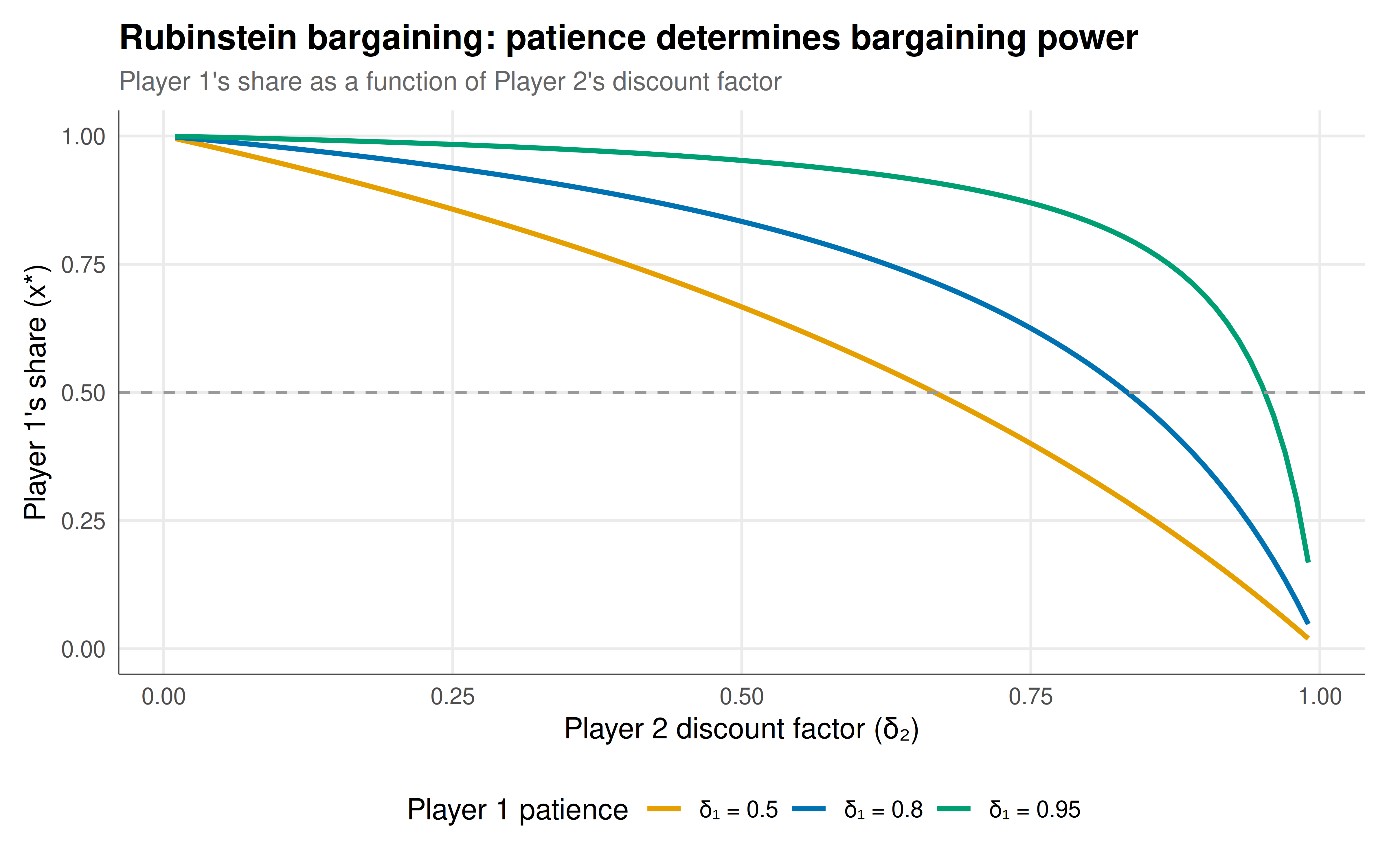
#| fig-cap: "Figure 1. Rubinstein bargaining outcomes as a function of Player 2's discount factor, for three levels of Player 1's patience. More patient players capture larger shares: when δ1 > δ2, Player 1 takes the lion's share. The dashed line marks the equal-split benchmark. As both players become very patient, shares converge to 50-50 regardless of asymmetry, recovering the Nash bargaining solution. Okabe-Ito palette."
#| dev: [png, pdf]
#| fig-width: 8
#| fig-height: 5
#| dpi: 300
delta2_seq <- seq(0.01, 0.99, by = 0.01)
patience_df <- lapply(c(0.5, 0.8, 0.95), function(d1) {
  shares <- sapply(delta2_seq, function(d2) rubinstein_spe(d1, d2)$x1_share)
  tibble(delta2 = delta2_seq, p1_share = shares, delta1 = paste0("δ₁ = ", d1))
}) |> bind_rows()

ggplot(patience_df, aes(x = delta2, y = p1_share, color = delta1)) +
  geom_line(linewidth = 1) +
  geom_hline(yintercept = 0.5, linetype = "dashed", color = "grey60") +
  scale_color_manual(values = okabe_ito[c(1, 5, 3)], name = "Player 1 patience") +
  labs(title = "Rubinstein bargaining: patience determines bargaining power",
       subtitle = "Player 1's share as a function of Player 2's discount factor",
       x = "Player 2 discount factor (δ₂)", y = "Player 1's share (x*)") +
  coord_cartesian(ylim = c(0, 1)) +
  theme_publication()
```
## Interactive figure
```{r}
#| label: fig-rubinstein-heatmap
# Heatmap of Player 1's share across (δ1, δ2) space
grid_df <- expand.grid(delta1 = seq(0.1, 0.99, by = 0.02),
                        delta2 = seq(0.1, 0.99, by = 0.02)) |>
  mutate(
    p1_share = (1 - delta2) / (1 - delta1 * delta2),
    text = paste0("δ₁ = ", round(delta1, 2), ", δ₂ = ", round(delta2, 2),
                  "\nP1 share: ", round(p1_share, 3),
                  "\nP2 share: ", round(1 - p1_share, 3))
  )

p_heat <- ggplot(grid_df, aes(x = delta1, y = delta2, fill = p1_share, text = text)) +
  geom_tile() +
  scale_fill_gradient2(low = okabe_ito[5], mid = "white", high = okabe_ito[6],
                        midpoint = 0.5, name = "P1 share") +
  geom_abline(slope = 1, intercept = 0, linetype = "dashed", color = "grey40") +
  labs(title = "Player 1's equilibrium share — Rubinstein bargaining",
       subtitle = "Above diagonal (δ₁ > δ₂): P1 more patient → gets more. Diagonal = symmetric.",
       x = "Player 1 discount factor (δ₁)", y = "Player 2 discount factor (δ₂)") +
  coord_equal() +
  theme_publication()

ggplotly(p_heat, tooltip = "text") |>
  config(displaylogo = FALSE, modeBarButtonsToRemove = c("select2d", "lasso2d"))
```
## Interpretation
Rubinstein's model provides the definitive non-cooperative theory of bilateral bargaining, and its predictions are remarkably clean: the unique SPE involves immediate agreement, with surplus division determined entirely by the players' relative patience. Patient players have more bargaining power because they can more credibly threaten to reject an offer and wait — the threat of delay is the source of all leverage. The first-mover advantage ($x^* = 1/(1+\delta) > 1/2$ in the symmetric case) reflects the fact that the proposer can exploit the responder's impatience: accepting now is worth more than making a counter-offer next period. But this advantage vanishes as $\delta \to 1$ (frequent offers, patient players), converging to the 50-50 Nash bargaining solution — providing the celebrated non-cooperative foundation for Nash's axiomatic theory. The heatmap reveals the full strategic landscape: above the diagonal ($\delta_1 > \delta_2$), Player 1 dominates; below, Player 2 dominates; and on the diagonal, the outcome is symmetric (modulo the vanishing first-mover advantage). In applications, the discount factor captures not just time preference but outside options, risk of breakdown, and institutional constraints: a union with a strike fund (high $\delta$) bargains better; a defendant facing mounting legal costs (low $\delta$) settles for less. The model also explains why bargaining breakdowns (strikes, wars, litigation) are puzzling from a rational perspective: in the complete-information model, delay never occurs. Breakdowns require additional ingredients — incomplete information about the opponent's patience, commitment problems, or multiple equilibria — which is why extensions like the Myerson-Satterthwaite theorem and mechanism design approach are essential complements to Rubinstein's foundational result.
## Extensions & related tutorials
- [Nash bargaining solution](../../foundations/nash-bargaining-solution/) — the axiomatic approach that Rubinstein microfounds.
- [Extensive-form games and subgame perfection](../../foundations/extensive-form-subgame-perfection/) — the equilibrium concept used here.
- [Ultimatum game and fairness](../../behavioral-gt/ultimatum-game-fairness/) — finite-round bargaining with fairness preferences.
- [Signaling games and PBE](../../foundations/signaling-games-pbe/) — bargaining under incomplete information.
- [Folk theorem with perfect monitoring](../../foundations/folk-theorem-perfect-monitoring/) — repeated interaction and patience.
## References
::: {#refs}
:::