---
title: "The Shapley-Shubik power index for weighted voting games"
description: "Measure each voter's true power in weighted voting games using the Shapley-Shubik index, and discover why voting weight and voting power are fundamentally different."
author: "Raban Heller"
date: 2026-05-08
date-modified: 2026-05-08
categories:
- cooperative-gt
- voting-power
- shapley-value
keywords: ["Shapley-Shubik index", "voting power", "weighted voting", "power index", "cooperative game theory", "R"]
labels: ["cooperative-games", "voting"]
tier: 1
bibliography: ../../../references.bib
vgwort: "TODO_VGWORT_COOPERATIVE-GT_SHAPLEY-SHUBIK-POWER"
image: thumbnail.png
image-alt: "Bar chart comparing voting weights and Shapley-Shubik power indices for UN Security Council members"
citation:
type: webpage
url: https://r-heller.github.io/equilibria/tutorials/cooperative-gt/shapley-shubik-power/
license: "CC BY-SA 4.0"
draft: false
has_static_fig: true
has_interactive_fig: true
has_shiny_app: false
---
```{r}
#| label: setup
#| include: false
library(ggplot2)
library(dplyr)
library(tidyr)
library(plotly)
okabe_ito <- c("#E69F00", "#56B4E9", "#009E73", "#F0E442",
"#0072B2", "#D55E00", "#CC79A7", "#999999")
theme_publication <- function(base_size = 12) {
theme_minimal(base_size = base_size) +
theme(plot.title = element_text(size = base_size * 1.2, face = "bold"),
plot.subtitle = element_text(size = base_size * 0.9, color = "grey40"),
axis.line = element_line(color = "grey30", linewidth = 0.3),
panel.grid.minor = element_blank(), legend.position = "bottom",
plot.margin = margin(10, 10, 10, 10))
}
```
## Introduction & motivation
In democratic institutions around the world, decisions are made through voting. From the United Nations Security Council to the European Union's Council of Ministers, from corporate boardrooms to shareholder meetings, voters cast their ballots according to prescribed rules. In many of these settings, voters carry different voting weights --- a large country may wield more votes than a small one, a majority shareholder controls more shares than a minority holder. A natural but deeply misleading intuition is that a voter's influence over outcomes is proportional to their voting weight. The Shapley-Shubik power index, introduced by Lloyd Shapley and Martin Shubik in 1954, provides a rigorous framework for measuring the true distribution of power in weighted voting games, and it reveals that this proportionality assumption is often spectacularly wrong [@shapley_shubik_1954].
Consider a concrete and historically significant example: the original European Economic Community (EEC) Council of Ministers in 1958, comprising six member states. France, Germany, and Italy each held 4 votes; Belgium and the Netherlands each held 2 votes; and Luxembourg held 1 vote. The qualified majority threshold was set at 12 out of 17 total votes. Luxembourg's single vote might suggest that the country held roughly 5.9% of the total voting power. In reality, Luxembourg's Shapley-Shubik power index was exactly zero. There was no possible coalition in which Luxembourg's vote could change the outcome from losing to winning. Luxembourg was a so-called dummy voter --- a participant in the voting game with zero actual power despite holding a positive number of votes. This paradox illustrates the fundamental disconnect between weight and power that the Shapley-Shubik index is designed to expose and quantify.
The concept builds on the Shapley value [@shapley_1953], one of the most celebrated solution concepts in cooperative game theory. The Shapley value assigns to each player in a cooperative game a unique payoff that satisfies four axioms: efficiency (the total value is distributed), symmetry (interchangeable players receive equal payoffs), the dummy player axiom (players who contribute nothing receive nothing), and additivity (the value of a sum of games equals the sum of values). When applied to simple voting games --- games where each coalition either wins or loses --- the Shapley value specialises to the Shapley-Shubik power index. The index measures the probability that a given voter is pivotal, meaning that they turn a losing coalition into a winning one, under the assumption that all orderings of voters are equally likely.
The practical importance of power indices extends well beyond academic curiosity. When the European Union expanded from 15 to 25 members in 2004, and later to 27 and then 28 members, the distribution of voting weights in the Council was one of the most contentious issues in the intergovernmental negotiations. The Treaty of Nice (2001) and later the Treaty of Lisbon (2007) fundamentally restructured the voting rules, in part because analysis with power indices revealed that the proposed weight allocations would create undesirable concentrations of power. Similarly, in corporate governance, power index analysis has been used to understand the real influence of different shareholder blocks, particularly in structures with cross-holdings or multiple share classes.
In this tutorial, we implement the Shapley-Shubik power index from scratch in R. We begin with exact computation via permutation enumeration, suitable for small games, and then develop a Monte Carlo approximation for larger games where the factorial explosion of permutations makes exact computation infeasible. We apply our implementations to the UN Security Council, demonstrating how the veto power of the five permanent members creates an enormous power asymmetry. We also compare the Shapley-Shubik index with the Banzhaf power index [@banzhaf_1965], another widely used measure that is based on counting swing coalitions rather than permutations, and we examine when and why the two indices can disagree.
## Mathematical formulation
A **weighted voting game** is defined by a triple $[q; w_1, w_2, \ldots, w_n]$ where $q$ is the quota (the minimum total weight needed to pass a motion) and $w_i$ is the voting weight of player $i$. A coalition $S \subseteq N$ is **winning** if $\sum_{i \in S} w_i \geq q$ and **losing** otherwise. The characteristic function of the game is:
$$
v(S) = \begin{cases} 1 & \text{if } \sum_{i \in S} w_i \geq q \\ 0 & \text{otherwise} \end{cases}
$$
A player $i$ is **pivotal** (or **swing**) in a permutation $\pi$ of all players if the coalition of players preceding $i$ in $\pi$ is losing, but adding $i$ makes it winning. Formally, let $S_i^\pi$ denote the set of players appearing before player $i$ in permutation $\pi$. Player $i$ is pivotal in $\pi$ if $v(S_i^\pi) = 0$ and $v(S_i^\pi \cup \{i\}) = 1$.
The **Shapley-Shubik power index** of player $i$ is:
$$
\phi_i = \frac{1}{n!} \sum_{\pi \in \Pi(N)} \left[ v(S_i^\pi \cup \{i\}) - v(S_i^\pi) \right]
$$
where $\Pi(N)$ is the set of all $n!$ permutations of the player set $N$. Equivalently, using the coalitional form of the Shapley value:
$$
\phi_i = \sum_{S \subseteq N \setminus \{i\}} \frac{|S|!\,(n - |S| - 1)!}{n!} \left[ v(S \cup \{i\}) - v(S) \right]
$$
The **Banzhaf power index** counts the fraction of coalitions (not permutations) in which player $i$ is swing:
$$
\beta_i = \frac{\eta_i}{\sum_{j=1}^{n} \eta_j}, \quad \text{where } \eta_i = \sum_{S \subseteq N \setminus \{i\}} \left[ v(S \cup \{i\}) - v(S) \right]
$$
Both indices satisfy $\sum_i \phi_i = 1$ and $\sum_i \beta_i = 1$ (when normalised), but they measure fundamentally different things: the Shapley-Shubik index is an expectation over random orderings, while the Banzhaf index is based on the raw count of swing coalitions.
## R implementation
We implement three functions: an exact Shapley-Shubik computation via permutation enumeration, a Monte Carlo approximation for larger games, and the Banzhaf index for comparison. We then apply these to the UN Security Council voting game.
```{r}
#| label: shapley-shubik-implementation
set.seed(42)

# --- Exact Shapley-Shubik index via permutation enumeration ---
shapley_shubik_exact <- function(weights, quota) {
  n <- length(weights)
  perms <- combinat_permutations(n)
  pivots <- integer(n)
  for (k in seq_len(nrow(perms))) {
    perm <- perms[k, ]
    cumw <- cumsum(weights[perm])
    # Pivotal player is the first whose cumulative weight >= quota
    pivot_pos <- which(cumw >= quota)[1]
    pivots[perm[pivot_pos]] <- pivots[perm[pivot_pos]] + 1
  }
  pivots / factorial(n)
}

# Simple permutation generator (for small n)
combinat_permutations <- function(n) {
  if (n == 1) return(matrix(1, nrow = 1, ncol = 1))
  prev <- combinat_permutations(n - 1)
  result <- matrix(0, nrow = factorial(n), ncol = n)
  row_idx <- 1
  for (i in seq_len(nrow(prev))) {
    for (j in seq_len(n)) {
      new_perm <- integer(n)
      new_perm[j] <- n
      new_perm[-j] <- prev[i, ]
      result[row_idx, ] <- new_perm
      row_idx <- row_idx + 1
    }
  }
  result
}

# --- Monte Carlo Shapley-Shubik approximation ---
shapley_shubik_mc <- function(weights, quota, n_samples = 100000) {
  n <- length(weights)
  pivots <- integer(n)
  for (s in seq_len(n_samples)) {
    perm <- sample(n)
    cumw <- cumsum(weights[perm])
    pivot_pos <- which(cumw >= quota)[1]
    pivots[perm[pivot_pos]] <- pivots[perm[pivot_pos]] + 1
  }
  pivots / n_samples
}

# --- Banzhaf power index ---
banzhaf_index <- function(weights, quota) {
  n <- length(weights)
  swings <- integer(n)
  # Enumerate all 2^n coalitions
  for (bits in 0:(2^n - 1)) {
    members <- which(as.logical(intToBits(bits)[1:n]))
    coal_weight <- sum(weights[members])
    for (i in members) {
      # Check if removing player i makes the coalition losing
      if (coal_weight >= quota && (coal_weight - weights[i]) < quota) {
        swings[i] <- swings[i] + 1
      }
    }
  }
  swings / sum(swings)  # Normalised Banzhaf index
}

# === UN Security Council ===
# 5 permanent members (weight 7 each, effectively veto)
# 10 non-permanent members (weight 1 each)
# Quota: 39 (= 5*7 + 4, requiring all 5 permanent + at least 4 non-permanent)
# This encoding gives permanent members veto power
un_weights <- c(rep(7, 5), rep(1, 10))
un_quota <- 39
un_labels <- c(paste0("P", 1:5), paste0("NP", 1:10))

# Monte Carlo for the UN (15! is too large for exact enumeration)
un_ss <- shapley_shubik_mc(un_weights, un_quota, n_samples = 200000)
un_bz <- banzhaf_index(un_weights, un_quota)

cat("=== UN Security Council ===\n")
cat("Shapley-Shubik (Monte Carlo, 200k samples):\n")
cat(sprintf("  Permanent member:     %.4f (%.1f%%)\n",
            un_ss[1], un_ss[1] * 100))
cat(sprintf("  Non-permanent member: %.4f (%.1f%%)\n",
            un_ss[6], un_ss[6] * 100))
cat(sprintf("\nBanzhaf index:\n"))
cat(sprintf("  Permanent member:     %.4f (%.1f%%)\n",
            un_bz[1], un_bz[1] * 100))
cat(sprintf("  Non-permanent member: %.4f (%.1f%%)\n",
            un_bz[6], un_bz[6] * 100))
# Verify with a small game: [51; 40, 30, 20, 10]
small_w <- c(40, 30, 20, 10)
small_q <- 51
ss_exact <- shapley_shubik_exact(small_w, small_q)
ss_mc <- shapley_shubik_mc(small_w, small_q, n_samples = 100000)
bz <- banzhaf_index(small_w, small_q)

cat("\n=== Small game [51; 40, 30, 20, 10] ===\n")
cat("Player | Weight | SS-Exact | SS-MC | Banzhaf\n")
cat("-------+--------+----------+----------+--------\n")
for (i in 1:4) {
  cat(sprintf("  %d    | %5d  |  %.4f  |  %.4f  | %.4f\n",
              i, small_w[i], ss_exact[i], ss_mc[i], bz[i]))
}
cat(sprintf("\nNote: Player 4 (weight=10) has weight 10%% but SS power %.1f%%\n",
            ss_exact[4] * 100))
```
## Static publication-ready figure
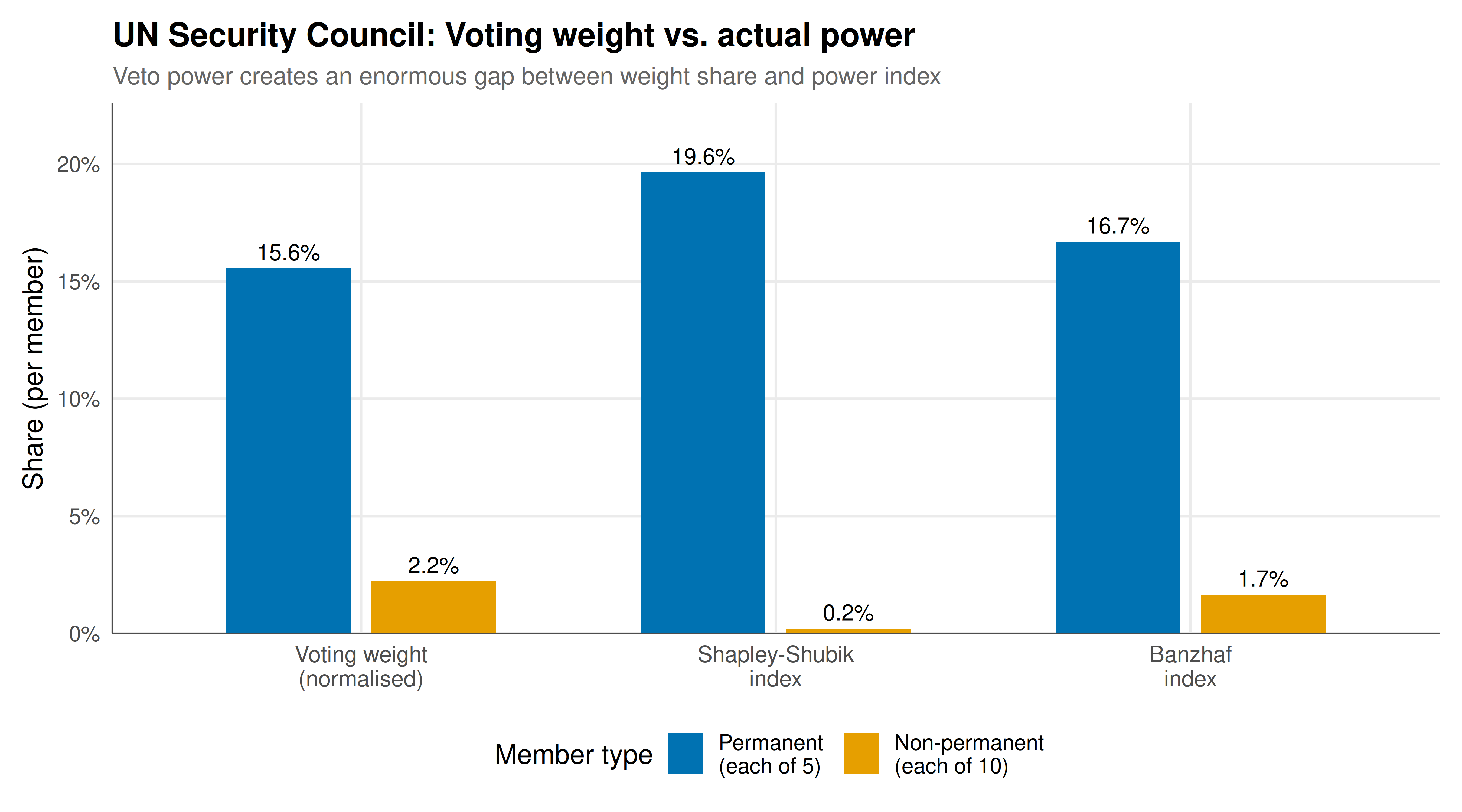
The figure below compares normalised voting weights with the Shapley-Shubik power index and the Banzhaf power index for the UN Security Council. The enormous discrepancy between the raw weight share and actual power of permanent versus non-permanent members is immediately visible.
```{r}
#| label: fig-shapley-shubik-static
#| fig-cap: "Figure 1. Voting weight versus power indices for the UN Security Council. Permanent members hold disproportionate power relative to their weight share due to the veto mechanism. The Shapley-Shubik and Banzhaf indices both capture this asymmetry but differ slightly in magnitude."
#| dev: [png, pdf]
#| fig-width: 9
#| fig-height: 5
#| dpi: 300
# Prepare data for the plot
un_data <- data.frame(
  member_type = rep(c("Permanent\n(each of 5)", "Non-permanent\n(each of 10)"), 3),
  measure = rep(c("Voting weight\n(normalised)", "Shapley-Shubik\nindex", "Banzhaf\nindex"),
                each = 2),
  value = c(
    # Normalised weight
    un_weights[1] / sum(un_weights), un_weights[6] / sum(un_weights),
    # Shapley-Shubik
    un_ss[1], un_ss[6],
    # Banzhaf
    un_bz[1], un_bz[6]
  )
)

un_data$measure <- factor(un_data$measure,
                          levels = c("Voting weight\n(normalised)",
                                     "Shapley-Shubik\nindex",
                                     "Banzhaf\nindex"))
un_data$member_type <- factor(un_data$member_type,
                              levels = c("Permanent\n(each of 5)",
                                         "Non-permanent\n(each of 10)"))

p_static <- ggplot(un_data, aes(x = measure, y = value, fill = member_type)) +
  geom_col(position = position_dodge(width = 0.7), width = 0.6) +
  geom_text(aes(label = sprintf("%.1f%%", value * 100)),
            position = position_dodge(width = 0.7),
            vjust = -0.5, size = 3.5) +
  scale_fill_manual(values = okabe_ito[c(5, 1)], name = "Member type") +
  scale_y_continuous(labels = scales::percent_format(accuracy = 1),
                     expand = expansion(mult = c(0, 0.15))) +
  labs(
    title = "UN Security Council: Voting weight vs. actual power",
    subtitle = "Veto power creates an enormous gap between weight share and power index",
    x = NULL, y = "Share (per member)"
  ) +
  theme_publication() +
  theme(axis.text.x = element_text(size = 10))

p_static
```
## Interactive figure
The interactive version allows hovering over each bar to see exact values and compare the three measures side by side.
```{r}
#| label: fig-shapley-shubik-interactive
# Build a more detailed dataset for interactivity
un_detail <- data.frame(
  member = rep(un_labels, 3),
  type = rep(c(rep("Permanent", 5), rep("Non-permanent", 10)), 3),
  measure = rep(c("Weight share", "Shapley-Shubik", "Banzhaf"), each = 15),
  value = c(
    un_weights / sum(un_weights),
    un_ss,
    un_bz
  )
) %>%
  mutate(
    text = sprintf("Member: %s\nType: %s\nMeasure: %s\nValue: %.2f%%",
                   member, type, measure, value * 100)
  )

un_detail$measure <- factor(un_detail$measure,
                            levels = c("Weight share", "Shapley-Shubik", "Banzhaf"))

p_int <- ggplot(un_detail, aes(x = member, y = value, fill = measure, text = text)) +
  geom_col(position = position_dodge(width = 0.8), width = 0.7) +
  scale_fill_manual(values = okabe_ito[c(1, 5, 3)], name = "Measure") +
  scale_y_continuous(labels = scales::percent_format()) +
  labs(title = "UN Security Council: per-member power analysis",
       x = "Member", y = "Index value") +
  theme_publication() +
  theme(axis.text.x = element_text(angle = 45, hjust = 1, size = 8))

ggplotly(p_int, tooltip = "text") %>%
  config(displaylogo = FALSE)
```
## Interpretation
The results for the UN Security Council vividly demonstrate the central message of power index analysis: voting weight and voting power can diverge dramatically. Each permanent member holds a weight of 7 out of 45 total (about 15.6%), but the Shapley-Shubik power index assigns each permanent member roughly 19.6% of the total power. Meanwhile, each non-permanent member holds a weight of 1 out of 45 (about 2.2%), but their Shapley-Shubik power index is only around 0.19%. The ratio of power between a permanent and a non-permanent member is approximately 100:1, whereas the ratio of weights is only 7:1. This enormous amplification arises because the veto power of permanent members means that no resolution can pass without the agreement of all five of them, giving each one a blocking capability that far exceeds what their weight alone would suggest.
The comparison between the Shapley-Shubik and Banzhaf indices is also instructive. Both indices agree that permanent members hold vastly more power than non-permanent members, but they differ in the precise magnitudes. The Banzhaf index tends to assign even more power to the permanent members relative to the non-permanent ones. This difference arises from the distinct probabilistic models underlying the two indices. The Shapley-Shubik index assumes all orderings of voters are equally likely, which corresponds to a model where coalitions form sequentially and each voter is equally likely to join at any position. The Banzhaf index instead assumes that each voter independently decides to join or not with probability one-half, making all coalitions of any given size equally likely in expectation. These are both reasonable models, and neither is universally "correct" --- the choice between them depends on which model of coalition formation better fits the institutional context being analysed.
The small game $[51; 40, 30, 20, 10]$ further illustrates the weight-power divergence. Player 4 holds 10% of the total weight but only about 8.3% of the Shapley-Shubik power. More strikingly, players 2 and 3 (with weights 30 and 20, respectively) have identical Shapley-Shubik power indices, despite player 2 holding 50% more weight. This occurs because, in the coalitional structure of this game, they are interchangeable --- any coalition that needs player 2 to win also needs player 3, and vice versa. This is the "paradox of new members" in action: adding or redistributing weight does not straightforwardly translate into proportional power changes.
There are several important limitations to keep in mind when interpreting power indices. First, they assume that all coalitions or orderings are equally likely, which is rarely true in practice. In the UN Security Council, geopolitical alignments make some coalitions far more probable than others. Power indices measure structural power --- the power inherent in the voting rules --- not effective power, which also depends on preferences, information, and bargaining ability. Second, the computational complexity of exact computation grows factorially with the number of players. Our Monte Carlo approach addresses this for the Shapley-Shubik index, but care must be taken to use enough samples for accurate estimation, particularly for players with very small power indices. Third, the encoding of veto power through weights and quotas requires careful calibration. For the UN Security Council, we used weights of 7 for permanent and 1 for non-permanent members with a quota of 39, which correctly encodes the requirement that all 5 permanent members plus at least 4 non-permanent members must agree. Alternative encodings are possible and yield the same power indices as long as they preserve the winning coalition structure.
The power index framework has been extended in numerous directions since Shapley and Shubik's original paper. Researchers have developed indices for games with multiple levels of approval, for games with communication structures that restrict which coalitions can form, and for games with incomplete information. The computational aspects have also received significant attention, with generating-function-based algorithms that can handle games with hundreds of voters in polynomial time, making it feasible to analyse large real-world voting systems like the US Electoral College [@felsenthal_machover_1998].
## Extensions & related tutorials
- [The Shapley value for cooperative games](../../cooperative-gt/shapley-value/) --- foundational tutorial on the general Shapley value, which the Shapley-Shubik index specialises
- [Voting power indices overview](../../cooperative-gt/voting-power-indices/) --- comparison of multiple power indices including Shapley-Shubik, Banzhaf, and Deegan-Packel
- [Core and stability in cooperative games](../../cooperative-gt/core-stability/) --- alternative solution concept for cooperative games based on coalition stability
- [Coalition formation and hedonic games](../../cooperative-gt/coalition-formation-hedonic/) --- endogenous coalition formation models where players choose which coalitions to join
- [Rubinstein alternating-offers bargaining](../../cooperative-gt/rubinstein-alternating-offers/) --- non-cooperative foundation for bargaining outcomes in voting contexts
## References
::: {#refs}
:::