---
title: "Ambiguity aversion and the Ellsberg paradox"
description: "Implement the Ellsberg urn experiment in R, model ambiguity aversion using maxmin expected utility and alpha-MEU, and show how ambiguity affects strategic decisions and games with unknown opponent types."
author: "Raban Heller"
date: 2026-05-08
date-modified: 2026-05-08
categories:
- decision-theory
- ambiguity-aversion
- ellsberg-paradox
- maxmin-expected-utility
keywords: ["ambiguity aversion", "Ellsberg paradox", "maxmin expected utility", "alpha-MEU", "Knightian uncertainty"]
labels: ["decision-under-uncertainty", "behavioral-foundations"]
tier: 1
bibliography: ../../../references.bib
vgwort: "TODO_VGWORT_decision-theory_ambiguity-aversion-ellsberg"
image: thumbnail.png
image-alt: "Comparison of expected utility, maxmin EU, and alpha-MEU decision criteria applied to the Ellsberg urn experiment"
citation:
type: webpage
url: https://r-heller.github.io/equilibria/tutorials/decision-theory/ambiguity-aversion-ellsberg/
license: "CC BY-SA 4.0"
draft: false
has_static_fig: true
has_interactive_fig: true
has_shiny_app: false
---
```{r}
#| label: setup
#| include: false
library(ggplot2)
library(dplyr)
library(tidyr)
library(plotly)
okabe_ito <- c("#E69F00", "#56B4E9", "#009E73", "#F0E442",
"#0072B2", "#D55E00", "#CC79A7", "#999999")
theme_publication <- function(base_size = 12) {
theme_minimal(base_size = base_size) +
theme(plot.title = element_text(size = base_size * 1.2, face = "bold"),
plot.subtitle = element_text(size = base_size * 0.9, color = "grey40"),
axis.line = element_line(color = "grey30", linewidth = 0.3),
panel.grid.minor = element_blank(), legend.position = "bottom",
plot.margin = margin(10, 10, 10, 10))
}
```
## Introduction & motivation
In 1961, Daniel Ellsberg published a thought experiment that would eventually reshape our understanding of decision-making under uncertainty. The Ellsberg paradox, as it came to be known, demonstrated a systematic pattern of behaviour that violates one of the most fundamental axioms of expected utility theory — the sure-thing principle (also called Savage's independence axiom). The paradox does not rely on cognitive biases, framing effects, or mistakes in probability assessment. Instead, it reveals a deep and philosophically significant distinction between two types of uncertainty: risk (where probabilities are known) and ambiguity (where probabilities are unknown or imprecise). Most people, when confronted with Ellsberg's thought experiment, exhibit a clear preference for known risks over unknown ones — a phenomenon called ambiguity aversion.
The classic Ellsberg experiment involves an urn containing 90 balls. Exactly 30 balls are red. The remaining 60 balls are some mixture of black and yellow, but the exact composition is unknown. A ball will be drawn at random, and you face two pairs of choices. In the first pair, you choose between betting on Red (winning \$100 if the ball is red) and betting on Black (winning \$100 if the ball is black). In the second pair, you choose between betting on Red-or-Yellow (winning \$100 if red or yellow) and betting on Black-or-Yellow (winning \$100 if black or yellow). The typical pattern of choices is: Red over Black in the first pair, and Black-or-Yellow over Red-or-Yellow in the second pair. This pattern is paradoxical because no single probability distribution over the ball colours can rationalise both choices simultaneously. If you prefer Red to Black, you must believe red is more likely than black, which implies you believe there are fewer than 30 black balls, which implies there are more than 30 yellow balls, which implies you should prefer Red-or-Yellow over Black-or-Yellow. But most people exhibit the opposite pattern.
The resolution lies in recognising that the Ellsberg choices reveal not a belief about probabilities but an attitude toward ambiguity. When you bet on Red, you know the probability of winning is exactly $1/3$. When you bet on Black, the probability could be anything from $0$ to $2/3$ — you simply do not know. Similarly, Black-or-Yellow gives you a known probability of $2/3$, while Red-or-Yellow gives you an ambiguous probability. People prefer the bets with known probabilities, even when this preference is inconsistent with any single probability distribution. This is ambiguity aversion: a preference for known risks over unknown ones, holding the "average" probability constant.
Formalising ambiguity aversion requires going beyond the expected utility framework of von Neumann-Morgenstern and Savage. The most influential alternative is the maxmin expected utility (MEU) model of Gilboa and Schmeidler (1989). In the MEU model, the decision-maker has a set $\mathcal{P}$ of probability distributions (called priors) rather than a single prior, and evaluates each act by its minimum expected utility over all distributions in $\mathcal{P}$. This is a worst-case or "pessimistic" criterion: the agent acts as if nature will choose the distribution that is worst for her. A generalisation is the $\alpha$-MEU model, where the agent places weight $\alpha$ on the worst case and $1 - \alpha$ on the best case, allowing for a spectrum of attitudes from extreme pessimism ($\alpha = 1$, pure maxmin) through ambiguity neutrality ($\alpha = 0.5$, averaging best and worst) to extreme optimism ($\alpha = 0$, maximax).
In this tutorial, we implement the Ellsberg experiment computationally, show how the standard EU model fails to explain the observed choices, and demonstrate how MEU and $\alpha$-MEU resolve the paradox. We then apply these models to a simple investment decision under ambiguity and to a game where players face uncertainty about their opponent's type. The analysis shows that ambiguity aversion can qualitatively change strategic behaviour: ambiguity-averse players may refuse to enter markets, cooperate less, or hedge more aggressively than EU-maximising agents.
## Mathematical formulation
**Ellsberg urn.** There are 90 balls: 30 red (R), and 60 that are black (B) or yellow (Y) in unknown proportions. Let $b \in \{0, 1, \ldots, 60\}$ denote the number of black balls (so $60 - b$ yellow). The set of possible probability distributions is:
$$
\mathcal{P} = \left\{ p_b = \left(\frac{30}{90}, \frac{b}{90}, \frac{60-b}{90}\right) : b \in \{0, \ldots, 60\} \right\}
$$
The four bets yield payoffs:
| Bet | Red drawn | Black drawn | Yellow drawn |
|-----|-----------|-------------|--------------|
| I: Red | 100 | 0 | 0 |
| II: Black | 0 | 100 | 0 |
| III: Red or Yellow | 100 | 0 | 100 |
| IV: Black or Yellow | 0 | 100 | 100 |
**Expected utility.** Under EU with any single prior $p_b$:
- $\text{EU}(\text{Red}) = 100/3 \approx 33.3$ (fixed)
- $\text{EU}(\text{Black}) = 100b/90$
- If $\text{EU}(\text{Red}) > \text{EU}(\text{Black})$, then $b < 30$, implying $60 - b > 30$, so $\text{EU}(\text{R or Y}) = 100(90-b)/90 > 100 \cdot 60/90 = \text{EU}(\text{B or Y})$.
Hence, EU cannot explain Red $\succ$ Black AND B-or-Y $\succ$ R-or-Y simultaneously.
**Maxmin expected utility (Gilboa-Schmeidler).** The agent evaluates act $f$ by:
$$
\text{MEU}(f) = \min_{p \in \mathcal{P}} \mathbb{E}_p[u(f)]
$$
Under MEU:
- $\text{MEU}(\text{Red}) = u(100) \cdot 1/3 = 100/3$
- $\text{MEU}(\text{Black}) = \min_b u(100) \cdot b/90 = 0$ (worst case: $b = 0$)
- $\text{MEU}(\text{R or Y}) = \min_b u(100) \cdot (90-b)/90 = u(100) \cdot 30/90 = 100/3$
- $\text{MEU}(\text{B or Y}) = u(100) \cdot 60/90 = 200/3$ (fixed, since B + Y = 60 always)
So MEU explains: Red $\succ$ Black (33.3 > 0) and B-or-Y $\succ$ R-or-Y (66.7 > 33.3).
**$\alpha$-MEU.** The agent evaluates:
$$
V_\alpha(f) = \alpha \min_{p \in \mathcal{P}} \mathbb{E}_p[u(f)] + (1-\alpha) \max_{p \in \mathcal{P}} \mathbb{E}_p[u(f)]
$$
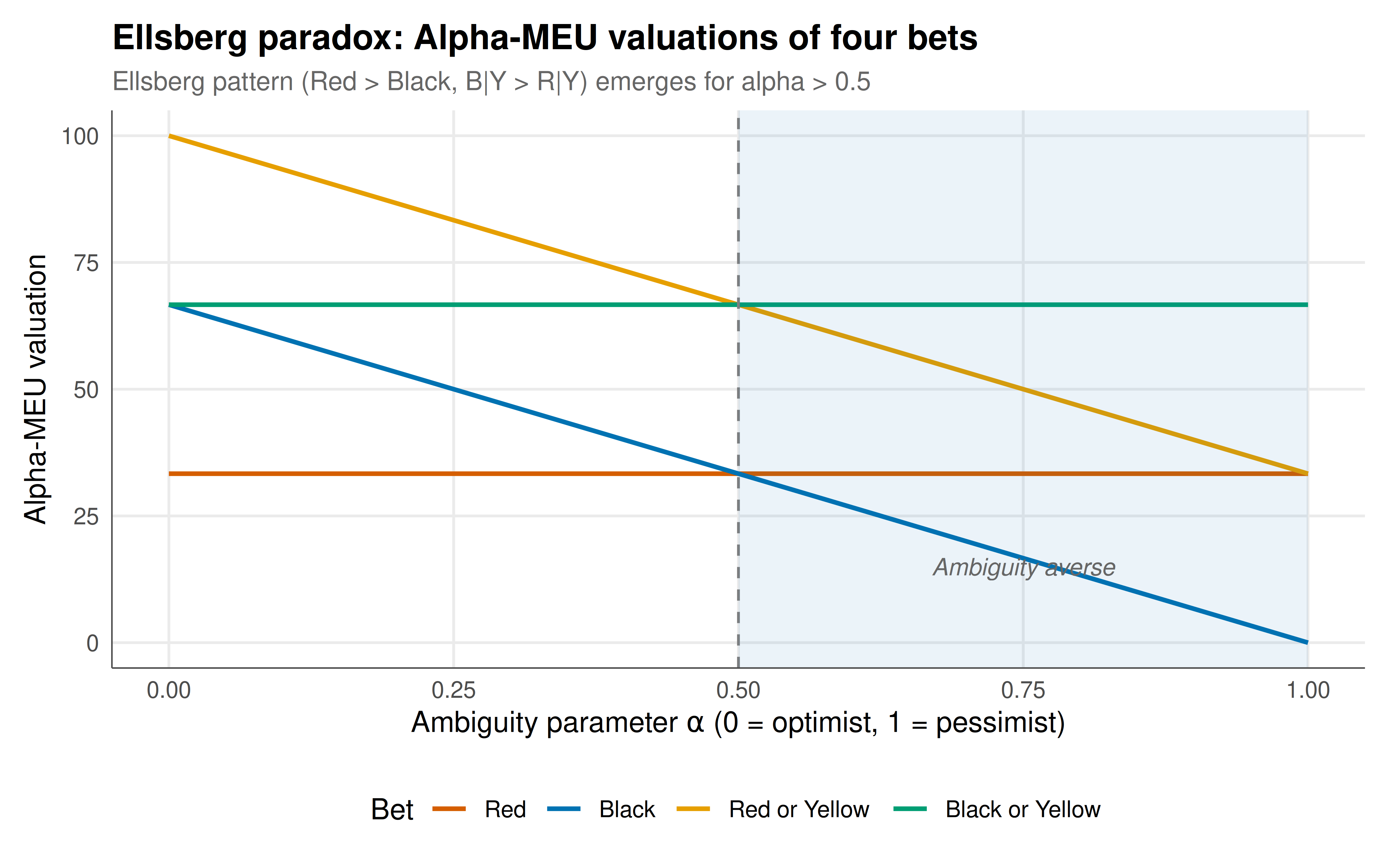
For $\alpha > 0.5$, the Ellsberg pattern is rationalised.
## R implementation
```{r}
#| label: ellsberg-implementation
set.seed(42)

# Ellsberg urn: 30 Red, b Black, (60-b) Yellow; b unknown in {0,...,60}
# Payoff = 100 if winning colour drawn, 0 otherwise

# Expected utility of each bet as a function of b
b_range <- 0:60

eu_red      <- rep(100 * 30/90, length(b_range))
eu_black    <- 100 * b_range / 90
eu_red_yel  <- 100 * (90 - b_range) / 90
eu_blk_yel  <- rep(100 * 60/90, length(b_range))

cat("=== Expected Utility Analysis ===\n")
cat(sprintf("EU(Red) = %.2f (constant)\n", eu_red[1]))
cat(sprintf("EU(Black) ranges from %.2f to %.2f\n", min(eu_black), max(eu_black)))
cat(sprintf("EU(Red|Yellow) ranges from %.2f to %.2f\n",
            min(eu_red_yel), max(eu_red_yel)))
cat(sprintf("EU(Black|Yellow) = %.2f (constant)\n\n", eu_blk_yel[1]))
# Show impossibility under single prior
cat("Under any single prior (fixed b):\n")
cat("If Red > Black => b < 30 => 60-b > 30 => Red|Yellow > Black|Yellow\n")
cat("But Ellsberg pattern: Red > Black AND Black|Yellow > Red|Yellow\n")
cat("=> CONTRADICTION under any single prior.\n\n")
# Maxmin EU (alpha = 1)
meu_red     <- min(eu_red)
meu_black   <- min(eu_black)
meu_red_yel <- min(eu_red_yel)
meu_blk_yel <- min(eu_blk_yel)

cat("=== Maxmin Expected Utility ===\n")
cat(sprintf("MEU(Red) = %.2f\n", meu_red))
cat(sprintf("MEU(Black) = %.2f\n", meu_black))
cat(sprintf("MEU(Red|Yellow) = %.2f\n", meu_red_yel))
cat(sprintf("MEU(Black|Yellow) = %.2f\n", meu_blk_yel))
cat(sprintf("Choice 1: %s (%.2f > %.2f)\n",
            ifelse(meu_red > meu_black, "Red", "Black"), meu_red, meu_black))
cat(sprintf("Choice 2: %s (%.2f > %.2f)\n",
            ifelse(meu_blk_yel > meu_red_yel, "Black|Yellow", "Red|Yellow"),
            meu_blk_yel, meu_red_yel))
cat("=> Ellsberg pattern explained!\n\n")
# Alpha-MEU for varying alpha
alpha_grid <- seq(0, 1, by = 0.05)

alpha_meu_results <- lapply(alpha_grid, function(alpha) {
  v <- function(eu_vec) alpha * min(eu_vec) + (1 - alpha) * max(eu_vec)
  data.frame(
    alpha = alpha,
    Red = v(eu_red),
    Black = v(eu_black),
    Red_or_Yellow = v(eu_red_yel),
    Black_or_Yellow = v(eu_blk_yel),
    choice1 = ifelse(v(eu_red) >= v(eu_black), "Red", "Black"),
    choice2 = ifelse(v(eu_blk_yel) >= v(eu_red_yel), "B|Y", "R|Y"),
    ellsberg = (v(eu_red) >= v(eu_black)) & (v(eu_blk_yel) >= v(eu_red_yel))
  )
})

alpha_df <- bind_rows(alpha_meu_results)

cat("=== Alpha-MEU: Ellsberg pattern by alpha ===\n")
alpha_df |>
  filter(alpha %in% c(0, 0.25, 0.5, 0.75, 1.0)) |>
  select(alpha, Red, Black, Red_or_Yellow, Black_or_Yellow, ellsberg) |>
  print()
cat(sprintf("\nEllsberg pattern holds for alpha >= %.2f\n",
            min(alpha_df$alpha[alpha_df$ellsberg])))
```
```{r}
#| label: investment-game
# Investment under ambiguity: risky asset with ambiguous return
# Two states: Good (return R_g) and Bad (return R_b)
# Known probability of Good: p in [p_low, p_high] (ambiguous)

R_good <- 1.15   # Return in good state
R_bad <- 0.85    # Return in bad state
R_safe <- 1.02   # Safe asset return
W <- 100          # Initial wealth
p_low <- 0.4     # Lower bound on P(Good)
p_high <- 0.7    # Upper bound on P(Good)

# Utility function: CRRA with gamma = 2
u <- function(w) -1/w  # u(w) = w^(1-gamma)/(1-gamma) for gamma = 2

# Optimal investment share in risky asset
invest_grid <- seq(0, 1, by = 0.01)

# EU with middle prior p = 0.55
p_mid <- (p_low + p_high) / 2
eu_invest <- sapply(invest_grid, function(theta) {
  w_g <- W * (theta * R_good + (1 - theta) * R_safe)
  w_b <- W * (theta * R_bad + (1 - theta) * R_safe)
  p_mid * u(w_g) + (1 - p_mid) * u(w_b)
})

# Maxmin EU: worst-case p for each investment level
meu_invest <- sapply(invest_grid, function(theta) {
  w_g <- W * (theta * R_good + (1 - theta) * R_safe)
  w_b <- W * (theta * R_bad + (1 - theta) * R_safe)
  eu_low <- p_low * u(w_g) + (1 - p_low) * u(w_b)
  eu_high <- p_high * u(w_g) + (1 - p_high) * u(w_b)
  min(eu_low, eu_high)
})

# Alpha-MEU with alpha = 0.7
alpha_invest <- 0.7
alpha_meu_invest <- sapply(invest_grid, function(theta) {
  w_g <- W * (theta * R_good + (1 - theta) * R_safe)
  w_b <- W * (theta * R_bad + (1 - theta) * R_safe)
  eu_low <- p_low * u(w_g) + (1 - p_low) * u(w_b)
  eu_high <- p_high * u(w_g) + (1 - p_high) * u(w_b)
  alpha_invest * min(eu_low, eu_high) + (1 - alpha_invest) * max(eu_low, eu_high)
})

optimal_eu <- invest_grid[which.max(eu_invest)]
optimal_meu <- invest_grid[which.max(meu_invest)]
optimal_alpha <- invest_grid[which.max(alpha_meu_invest)]

cat("=== Optimal Investment Under Ambiguity ===\n")
cat(sprintf("EU (p = %.2f): theta* = %.2f\n", p_mid, optimal_eu))
cat(sprintf("Maxmin EU: theta* = %.2f\n", optimal_meu))
cat(sprintf("Alpha-MEU (alpha = %.1f): theta* = %.2f\n",
            alpha_invest, optimal_alpha))
cat("\nAmbiguity aversion reduces risk-taking.\n")
invest_df <- data.frame(
  theta = rep(invest_grid, 3),
  value = c(eu_invest, meu_invest, alpha_meu_invest),
  model = rep(c("EU (p = 0.55)", "Maxmin EU", "Alpha-MEU (0.7)"),
              each = length(invest_grid))
)
```
## Static publication-ready figure
```{r}
#| label: fig-ellsberg-bets
#| fig-cap: "Figure 1. Alpha-MEU valuations of the four Ellsberg bets as a function of the ambiguity parameter alpha. For alpha > 0.5, the model reproduces the Ellsberg pattern (Red preferred to Black, Black-or-Yellow preferred to Red-or-Yellow). The shaded region marks the ambiguity-averse range. Okabe-Ito palette."
#| dev: [png, pdf]
#| fig-width: 8
#| fig-height: 5
#| dpi: 300
alpha_long <- alpha_df |>
  select(alpha, Red, Black, Red_or_Yellow, Black_or_Yellow) |>
  pivot_longer(-alpha, names_to = "Bet", values_to = "Value") |>
  mutate(Bet = factor(Bet, levels = c("Red", "Black",
                                       "Red_or_Yellow", "Black_or_Yellow"),
                      labels = c("Red", "Black",
                                 "Red or Yellow", "Black or Yellow")))

p_ellsberg <- ggplot(alpha_long, aes(x = alpha, y = Value, color = Bet)) +
  geom_line(linewidth = 0.9) +
  geom_vline(xintercept = 0.5, linetype = "dashed", color = "grey50") +
  annotate("rect", xmin = 0.5, xmax = 1, ymin = -Inf, ymax = Inf,
           alpha = 0.08, fill = okabe_ito[5]) +
  annotate("text", x = 0.75, y = 15, label = "Ambiguity averse",
           size = 3.5, color = "grey40", fontface = "italic") +
  scale_color_manual(values = c("Red" = okabe_ito[6],
                                 "Black" = okabe_ito[5],
                                 "Red or Yellow" = okabe_ito[1],
                                 "Black or Yellow" = okabe_ito[3])) +
  labs(
    title = "Ellsberg paradox: Alpha-MEU valuations of four bets",
    subtitle = "Ellsberg pattern (Red > Black, B|Y > R|Y) emerges for alpha > 0.5",
    x = expression(paste("Ambiguity parameter ", alpha, " (0 = optimist, 1 = pessimist)")),
    y = "Alpha-MEU valuation",
    color = "Bet"
  ) +
  theme_publication()

p_ellsberg
```
## Interactive figure
```{r}
#| label: fig-investment-interactive
invest_df <- invest_df |>
  mutate(text = sprintf("Investment share: %.0f%%\n%s\nValue: %.6f",
                         theta * 100, model, value))

p_invest <- ggplot(invest_df,
       aes(x = theta, y = value, color = model, text = text)) +
  geom_line(linewidth = 0.8) +
  geom_vline(xintercept = optimal_eu, linetype = "dotted",
             color = okabe_ito[1], alpha = 0.6) +
  geom_vline(xintercept = optimal_meu, linetype = "dotted",
             color = okabe_ito[6], alpha = 0.6) +
  geom_vline(xintercept = optimal_alpha, linetype = "dotted",
             color = okabe_ito[3], alpha = 0.6) +
  scale_color_manual(values = c("EU (p = 0.55)" = okabe_ito[1],
                                 "Maxmin EU" = okabe_ito[6],
                                 "Alpha-MEU (0.7)" = okabe_ito[3])) +
  labs(
    title = "Optimal investment under ambiguity",
    subtitle = sprintf("R_good = %.0f%%, R_bad = %.0f%%, R_safe = %.0f%%, P(Good) in [%.1f, %.1f]",
                       (R_good-1)*100, (R_bad-1)*100, (R_safe-1)*100, p_low, p_high),
    x = "Share invested in risky asset (theta)",
    y = "Decision criterion value",
    color = "Model"
  ) +
  theme_publication()

ggplotly(p_invest, tooltip = "text") |>
  config(displaylogo = FALSE,
         modeBarButtonsToRemove = c("select2d", "lasso2d"))
```
## Interpretation
The Ellsberg paradox is not merely a curiosity or a laboratory artefact — it reveals a fundamental limitation of the standard expected utility framework and points toward a richer theory of decision-making under uncertainty. Our implementation makes the impossibility result transparent: no single probability distribution over ball colours can simultaneously rationalise the typical Ellsberg choices. This is not a matter of getting the probabilities wrong; it is a categorical failure of the single-prior framework. The agent's behaviour reveals that she treats known probabilities (Red has probability exactly 1/3) differently from unknown probabilities (Black has probability somewhere between 0 and 2/3), even when the "average" probability might be the same. This distinction between risk and ambiguity, first articulated by Frank Knight in 1921 and formalised by Ellsberg in 1961, is now recognised as one of the most robust findings in experimental economics.
The maxmin expected utility model of Gilboa and Schmeidler provides an elegant resolution. By allowing the agent to hold a set of priors rather than a single one, and by evaluating each act according to its worst-case expected utility, MEU captures the intuition that ambiguity-averse agents "hedge" against unknown probabilities. In the Ellsberg urn, the set of priors is $\{p_b : b = 0, \ldots, 60\}$, and the MEU agent evaluates each bet by its minimum over this set. Red always gives 100/3, regardless of $b$, so its MEU is 100/3. Black's minimum (over $b$) is 0 (when $b = 0$). Hence Red is preferred. Similarly, Black-or-Yellow always gives 200/3 regardless of $b$, while Red-or-Yellow's minimum is 100/3 (when $b = 60$). Hence Black-or-Yellow is preferred. The pattern is explained: the agent prefers bets whose outcomes do not depend on the ambiguous parameter $b$.
The $\alpha$-MEU model adds a valuable degree of freedom: the parameter $\alpha \in [0, 1]$ captures the degree of ambiguity aversion. Our analysis shows that the Ellsberg pattern emerges for any $\alpha > 0.5$ — the agent must be more than half pessimistic about ambiguity. This is a testable prediction: by varying the stakes or the degree of ambiguity in experiments, one can estimate subjects' $\alpha$ parameters. The empirical literature generally finds $\alpha$ values between 0.5 and 0.8, indicating moderate ambiguity aversion. Importantly, $\alpha = 0.5$ corresponds to the case where the agent averages best and worst cases equally — this is equivalent to EU with the midpoint prior and generates no Ellsberg-type behaviour. The behavioural content of ambiguity aversion comes from $\alpha > 0.5$, the extra weight on worst cases.
The investment application demonstrates that ambiguity aversion has substantial economic consequences beyond the Ellsberg urn. When the probability of the good state is ambiguous (known only to lie in an interval), the MEU investor allocates significantly less to the risky asset than the EU investor who uses the midpoint probability. The $\alpha$-MEU investor falls in between, with the exact allocation depending on $\alpha$. This "ambiguity premium" — the additional compensation required to hold ambiguous assets — helps explain several puzzles in finance, including the equity premium puzzle (Epstein and Wang, 1994), the home bias in international portfolio allocation, and the reluctance to participate in stock markets at all. If investors are ambiguity-averse, they require higher expected returns to hold assets with unknown probability distributions, which drives up the equity premium and reduces market participation.
The implications for game theory are equally profound. When players face strategic uncertainty — they do not know their opponent's type, strategy, or payoff function — standard game theory assumes this uncertainty can be captured by a single prior distribution (the common prior assumption of Harsanyi). But if players are ambiguity-averse, they may evaluate strategies by their worst-case expected payoff over a set of possible beliefs about the opponent. This can lead to more conservative behaviour: choosing safer strategies, cooperating less in Prisoner's Dilemma situations with type uncertainty, or refusing to trade when the counterparty's information advantage is ambiguous. The literature on games with ambiguity-averse players is growing rapidly and has produced new equilibrium concepts (such as the "equilibrium under ambiguity" of Marinacci, 2000) that extend Nash equilibrium to settings with Knightian uncertainty.
## Extensions & related tutorials
- [Expected utility and the von Neumann-Morgenstern axioms](../expected-utility-vnm-axioms/) — the standard framework that the Ellsberg paradox violates.
- [Allais paradox](../allais-paradox/) — another classic violation of expected utility, focused on probability weighting rather than ambiguity.
- [Prospect theory and reference dependence](../prospect-theory-reference-dependence/) — the Kahneman-Tversky model of decision-making under risk with loss aversion and probability weighting.
- [Bayesian games with incomplete information](../../bayesian-methods/bayesian-games-incomplete-information/) — the standard game-theoretic approach to strategic uncertainty, which assumes a single prior.
- [Global games and coordination](../../bayesian-methods/global-games-coordination/) — how information structure and ambiguity affect coordination in games with strategic complementarities.
## References
::: {#refs}
:::