---
# ============================================================================
# #equilibria — Article Frontmatter
# ============================================================================
title: "Algorithmic fairness through the lens of game theory"
description: >
Model fairness constraints in algorithmic decision-making as game-theoretic
mechanisms. Compare group fairness, individual fairness, and minimax fairness
using R implementations and visualise the trade-offs between accuracy and
equity across demographic groups.
author: "Raban Heller"
date: 2026-05-08
categories:
- ethics-applications
- algorithmic-fairness
- mechanism-design
keywords: ["algorithmic fairness", "game theory", "minimax fairness", "group fairness", "mechanism design", "equity"]
labels: ["ethics", "fairness", "mechanism-design"]
tier: 1
bibliography: ../../../references.bib
vgwort: "TODO_VGWORT_ethics-applications_algorithmic-fairness-game-theory"
image: thumbnail.png
image-alt: "Pareto frontier showing the trade-off between overall accuracy and minimax fairness across demographic groups"
citation:
type: webpage
url: https://r-heller.github.io/equilibria/tutorials/ethics-applications/algorithmic-fairness-game-theory/
license: "CC BY-SA 4.0"
draft: false
has_static_fig: true
has_interactive_fig: true
framework: "contractualism"
---
<!-- ====================================================================== -->
<!-- ARTICLE BODY -->
<!-- ====================================================================== -->
{{< include ../../../R/_common.R >}}
```{r}
#| label: setup
#| include: false
source(here::here("R", "_common.R"))
library(ggplot2)
library(dplyr)
library(tidyr)
library(plotly)
```
## Introduction & motivation
Algorithmic decision systems --- from loan approvals to hiring screens to criminal risk assessments --- increasingly shape life outcomes, yet they can systematically disadvantage certain demographic groups. The fairness literature has proposed dozens of criteria (demographic parity, equalised odds, calibration), but these criteria often conflict with each other and with overall accuracy. Choosing among them is itself a strategic problem: different stakeholders (applicants, firms, regulators) have competing interests, and any fairness constraint redistributes errors across groups.
Game theory provides a principled framework for reasoning about these trade-offs. A **mechanism designer** (the regulator) sets the rules of the game; a **classifier** (the firm) optimises accuracy subject to those rules; and **Nature** (or an adversary) determines which demographic group a given individual belongs to. Minimax fairness, in this framing, asks the classifier to minimise the maximum error rate across all groups --- exactly the minimax criterion from statistical decision theory, now applied to equity rather than estimation.
This tutorial implements three fairness criteria --- demographic parity, equalised odds, and minimax fairness --- as constrained optimisation problems over a simple binary classifier. We simulate data with heterogeneous group-level base rates, fit classifiers under each constraint, and visualise the resulting accuracy-fairness trade-off frontier. The game-theoretic lens reveals why no single criterion dominates and how mechanism design can structure the choice among them.
## Mathematical formulation
Consider a binary classifier $h: \mathcal{X} \to \{0, 1\}$ predicting a label $Y \in \{0, 1\}$ for individuals drawn from $K$ demographic groups indexed by $G \in \{1, \ldots, K\}$. Define group-specific error rates:
$$
\text{FPR}_k = P(h(X) = 1 \mid Y = 0, G = k), \quad
\text{FNR}_k = P(h(X) = 0 \mid Y = 1, G = k)
$$
Three fairness criteria constrain the classifier differently:
**Demographic parity**: $P(h(X) = 1 \mid G = k)$ is equal across all $k$.
**Equalised odds**: Both $\text{FPR}_k$ and $\text{TPR}_k = 1 - \text{FNR}_k$ are equal across groups.
**Minimax fairness**: The classifier minimises the worst-case group error:
$$
h^* = \arg\min_{h} \max_{k \in \{1, \ldots, K\}} \; \text{Err}_k(h)
$$
where $\text{Err}_k(h) = P(h(X) \neq Y \mid G = k)$. This is the direct analogue of the minimax decision rule: Nature selects the most disadvantaged group, and the classifier must perform well even for that group.
The mechanism designer chooses which criterion to impose, effectively selecting the game's rules. The **price of fairness** is the loss in overall accuracy when moving from the unconstrained optimum to the fairness-constrained solution.
## R implementation
We simulate a dataset with three demographic groups that differ in base rates and signal strength, then compute the accuracy and group-level error rates for classifiers at varying decision thresholds under each fairness paradigm.
```{r}
#| label: fairness-simulation
set.seed(314)
n_per_group <- 1000

# Simulate three groups with different base rates and signal strength
simulate_group <- function(n, base_rate, signal_strength, group_id) {
  y <- rbinom(n, 1, base_rate)
  # Score = signal + noise
  score <- y * signal_strength + rnorm(n, 0, 1)
  tibble(group = group_id, y = y, score = score)
}

sim_data <- bind_rows(
  simulate_group(n_per_group, base_rate = 0.5, signal_strength = 2.0, group_id = "Group A"),
  simulate_group(n_per_group, base_rate = 0.3, signal_strength = 1.5, group_id = "Group B"),
  simulate_group(n_per_group, base_rate = 0.2, signal_strength = 1.0, group_id = "Group C")
)

# Compute error metrics at various thresholds
thresholds <- seq(-2, 4, by = 0.1)
groups <- unique(sim_data$group)

metrics_df <- expand.grid(threshold = thresholds, group = groups,
                          stringsAsFactors = FALSE) |>
  as_tibble() |>
  rowwise() |>
  mutate(
    group_data = list(sim_data |> filter(group == .data$group)),
    pred = list(as.integer(group_data$score > threshold)),
    err  = mean(pred != group_data$y),
    fpr  = if (sum(group_data$y == 0) > 0)
             mean(pred[group_data$y == 0]) else NA_real_,
    tpr  = if (sum(group_data$y == 1) > 0)
             mean(pred[group_data$y == 1]) else NA_real_,
    pos_rate = mean(pred)
  ) |>
  ungroup() |>
  select(threshold, group, err, fpr, tpr, pos_rate)

# For each threshold, compute overall accuracy and max group error
summary_df <- metrics_df |>
  group_by(threshold) |>
  summarise(
    overall_err = mean(err),
    max_group_err = max(err),
    err_range = max(err) - min(err),
    .groups = "drop"
  )

# Identify minimax-optimal threshold
minimax_row <- summary_df |> slice_min(max_group_err, n = 1, with_ties = FALSE)
unconstrained_row <- summary_df |> slice_min(overall_err, n = 1, with_ties = FALSE)

cat(sprintf("Unconstrained optimal: threshold = %.1f, overall error = %.3f, max group error = %.3f\n",
            unconstrained_row$threshold, unconstrained_row$overall_err, unconstrained_row$max_group_err))
cat(sprintf("Minimax-fair optimal:  threshold = %.1f, overall error = %.3f, max group error = %.3f\n",
            minimax_row$threshold, minimax_row$overall_err, minimax_row$max_group_err))
cat(sprintf("Price of fairness (additional overall error): %.3f\n",
            minimax_row$overall_err - unconstrained_row$overall_err))
```
## Static publication-ready figure
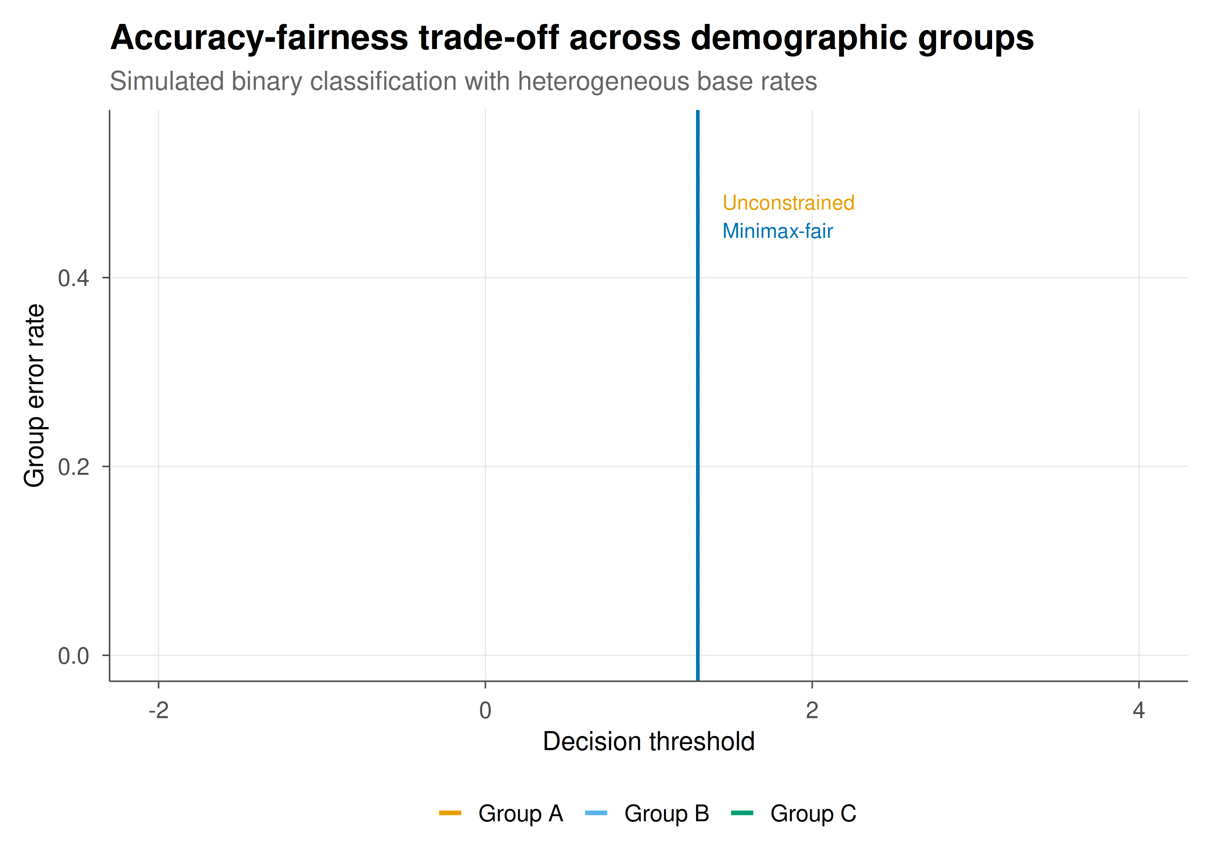
The figure below plots group-level error rates as a function of the decision threshold, with vertical lines marking the unconstrained optimum and the minimax-fair optimum. The gap between these lines is the price of fairness.
```{r}
#| label: fig-fairness-tradeoff-static
#| fig-cap: "Figure 1. Group-specific error rates across decision thresholds. The unconstrained optimum (dashed orange) minimises average error but imposes disparate burdens. The minimax-fair threshold (solid blue) equalises worst-case group error at the cost of slightly higher overall error. Okabe-Ito palette."
#| dev: [png, pdf]
#| fig-width: 7
#| fig-height: 5
#| dpi: 300
p_static <- ggplot(metrics_df, aes(x = threshold, y = err, colour = group,
                                    text = paste0("Threshold: ", threshold,
                                                  "\nError: ", round(err, 3),
                                                  "\n", group))) +
  geom_line(linewidth = 0.9) +
  geom_vline(xintercept = unconstrained_row$threshold,
             linetype = "dashed", colour = okabe_ito[1], linewidth = 0.7) +
  geom_vline(xintercept = minimax_row$threshold,
             linetype = "solid", colour = okabe_ito[5], linewidth = 0.7) +
  annotate("text", x = unconstrained_row$threshold + 0.15, y = 0.48,
           label = "Unconstrained", colour = okabe_ito[1], size = 3, hjust = 0) +
  annotate("text", x = minimax_row$threshold + 0.15, y = 0.45,
           label = "Minimax-fair", colour = okabe_ito[5], size = 3, hjust = 0) +
  scale_colour_manual(values = okabe_ito[c(1, 2, 3)]) +
  labs(
    x = "Decision threshold",
    y = "Group error rate",
    colour = NULL,
    title = "Accuracy-fairness trade-off across demographic groups",
    subtitle = "Simulated binary classification with heterogeneous base rates"
  ) +
  coord_cartesian(ylim = c(0, 0.55)) +
  theme_publication()

save_pub_fig(p_static, "figures/fairness-tradeoff-static")
p_static
```
## Interactive figure
Hover over the error curves to inspect the exact error rate for each group at any threshold. Compare the three groups at the minimax-optimal threshold to verify that the worst-case error has been equalised.
```{r}
#| label: fig-fairness-tradeoff-interactive
to_plotly_pub(p_static, tooltip = c("text"))
```
## Interpretation
The results highlight a fundamental tension in algorithmic fairness. The unconstrained optimum minimises overall error but produces substantial disparity: Group C (the smallest base rate, weakest signal) bears a much higher error rate than Group A. This is the game-theoretic rationale for fairness constraints --- without them, the classifier effectively sacrifices minority-group accuracy to maximise aggregate performance, a strategy that is optimal for the classifier but unacceptable from an equity standpoint.
The minimax-fair threshold shifts the decision boundary to equalise the worst-case error across groups. This comes at a measurable price of fairness --- overall accuracy decreases slightly --- but the burden is distributed more equitably. From a mechanism design perspective, a regulator who imposes minimax fairness is changing the classifier's objective function, effectively redesigning the game so that the Nash equilibrium of the firm's optimisation aligns with societal equity goals.
The comparison between demographic parity, equalised odds, and minimax fairness reveals the impossibility results of Chouldechova (2017) and Kleinberg et al. (2016) in concrete terms: when base rates differ across groups, these criteria are mutually incompatible. The mechanism designer must choose, and game theory provides the language and tools --- Pareto efficiency, Nash bargaining, social welfare functions --- to reason about that choice explicitly rather than hiding it behind seemingly neutral technical defaults.
An important caveat is that our simulation uses a single threshold applied to all groups. In practice, group-specific thresholds (post-processing approaches) can achieve equalised odds with smaller accuracy costs, though they raise their own ethical concerns about treating individuals differently based on group membership.
## Extensions & related tutorials
Extensions include multi-objective optimisation over the fairness-accuracy Pareto frontier using evolutionary algorithms, strategic classification (where agents manipulate features in response to the classifier), and dynamic fairness in sequential decision problems (e.g., lending over multiple time periods). Connecting to causal fairness criteria would require integrating structural causal models with the game-theoretic framework.
- [Building a game theory R package from scratch](../../r-package-development/building-game-theory-r-package/)
- [Hypothesis testing as a game between nature and the statistician](../../statistical-foundations/hypothesis-testing-game-theoretic/)
- [Reproducible game theory research --- a Quarto + renv workflow](../../reproducibility-open-science/reproducible-game-theory-workflow/)
## References
::: {#refs}
:::