---
# ============================================================================
# #equilibria — Article Frontmatter
# ============================================================================
title: "Hypothesis testing as a game between nature and the statistician"
description: >
Reframe classical hypothesis testing as a two-player minimax game in which
nature chooses the true state and the statistician selects a decision rule.
Derive the Neyman-Pearson lemma as the minimax optimal strategy and explore
power analysis as strategic optimisation.
author: "Raban Heller"
date: 2026-05-08
categories:
- statistical-foundations
- hypothesis-testing
- minimax
keywords: ["hypothesis testing", "minimax", "Neyman-Pearson", "power analysis", "game theory", "decision theory"]
labels: ["statistics", "minimax", "neyman-pearson"]
tier: 1
bibliography: ../../../references.bib
vgwort: "TODO_VGWORT_statistical-foundations_hypothesis-testing-game-theoretic"
image: thumbnail.png
image-alt: "ROC-style plot showing the trade-off between Type I and Type II error as a strategic frontier"
citation:
type: webpage
url: https://r-heller.github.io/equilibria/tutorials/statistical-foundations/hypothesis-testing-game-theoretic/
license: "CC BY-SA 4.0"
draft: false
has_static_fig: true
has_interactive_fig: true
---
<!-- ====================================================================== -->
<!-- ARTICLE BODY -->
<!-- ====================================================================== -->
{{< include ../../../R/_common.R >}}
```{r}
#| label: setup
#| include: false
source(here::here("R", "_common.R"))
library(ggplot2)
library(dplyr)
library(tidyr)
library(plotly)
```
## Introduction & motivation
Statisticians routinely talk about hypothesis tests in procedural terms: choose a significance level, compute a test statistic, compare to a critical value. But underneath this recipe lies a deep strategic structure. The data-generating process can be viewed as a move by Nature, who selects the true parameter value from the parameter space. The statistician responds by choosing a decision rule --- accept or reject the null hypothesis --- that minimises the worst-case error. This is precisely a two-player zero-sum game, and the minimax theorem guarantees the existence of an optimal strategy.
Viewing hypothesis testing through a game-theoretic lens clarifies several otherwise opaque concepts. The significance level $\alpha$ becomes a budget constraint on the statistician's strategy set. The Neyman--Pearson lemma emerges not as an ad-hoc optimality result but as the unique minimax solution for simple-versus-simple testing. Power analysis --- choosing sample sizes to achieve a target detection rate --- is revealed as a form of strategic resource allocation against an adversarial Nature who may place the true effect size at the hardest-to-detect value. This perspective unifies frequentist testing, Wald's statistical decision theory, and modern minimax estimation under a single conceptual roof.
This tutorial formalises the game, derives the optimal test as a likelihood ratio, and visualises the resulting trade-offs between Type I and Type II error across a range of effect sizes and sample sizes.
## Mathematical formulation
Define a two-player game $\Gamma = (\Theta, \mathcal{D}, L)$ where:
- **Nature** chooses $\theta \in \Theta = \{\theta_0, \theta_1\}$ (null vs. alternative),
- **Statistician** chooses a decision rule $\delta: \mathcal{X} \to \{0, 1\}$ from the set $\mathcal{D}$ of all measurable decision functions,
- **Loss** $L(\theta, \delta)$ penalises errors: $L(\theta_0, 1) = 1$ (Type I), $L(\theta_1, 0) = 1$ (Type II), and $L = 0$ otherwise.
The statistician's risk under $\theta$ is $R(\theta, \delta) = E_\theta[L(\theta, \delta(X))]$. The minimax decision rule solves:
$$
\delta^* = \arg\min_{\delta \in \mathcal{D}} \max_{\theta \in \Theta} R(\theta, \delta)
$$
For testing $H_0: X \sim N(\mu_0, \sigma^2)$ against $H_1: X \sim N(\mu_1, \sigma^2)$, the **Neyman--Pearson lemma** states that the most powerful test at level $\alpha$ rejects when the likelihood ratio exceeds a threshold:
$$
\Lambda(x) = \frac{f(x \mid \theta_1)}{f(x \mid \theta_0)} > k_\alpha
$$
The power of this test is:
$$
\beta(\mu_1) = P\!\left(\bar{X} > \mu_0 + z_{1-\alpha} \cdot \frac{\sigma}{\sqrt{n}} \;\middle|\; \mu = \mu_1\right)
= \Phi\!\left(\frac{\mu_1 - \mu_0}{\sigma / \sqrt{n}} - z_{1-\alpha}\right)
$$
## R implementation
We compute the power function across a grid of effect sizes $\delta = (\mu_1 - \mu_0) / \sigma$ and sample sizes $n$, visualising how the statistician's detection ability improves with more data.
```{r}
#| label: power-computation
alpha <- 0.05
z_alpha <- qnorm(1 - alpha)
effect_sizes <- seq(0.1, 1.5, by = 0.05)
sample_sizes <- c(10, 30, 50, 100, 200)

power_df <- expand.grid(delta = effect_sizes, n = sample_sizes) |>
  as_tibble() |>
  mutate(
    power = pnorm(delta * sqrt(n) - z_alpha),
    n_label = paste0("n = ", n)
  )

# Show a summary table for delta = 0.5
power_df |>
  filter(abs(delta - 0.5) < 0.01) |>
  select(n_label, delta, power) |>
  knitr::kable(
    digits = 3,
    col.names = c("Sample size", "Effect size (delta)", "Power"),
    caption = "Power at delta = 0.5 for various sample sizes (alpha = 0.05)"
  )
```
## Static publication-ready figure
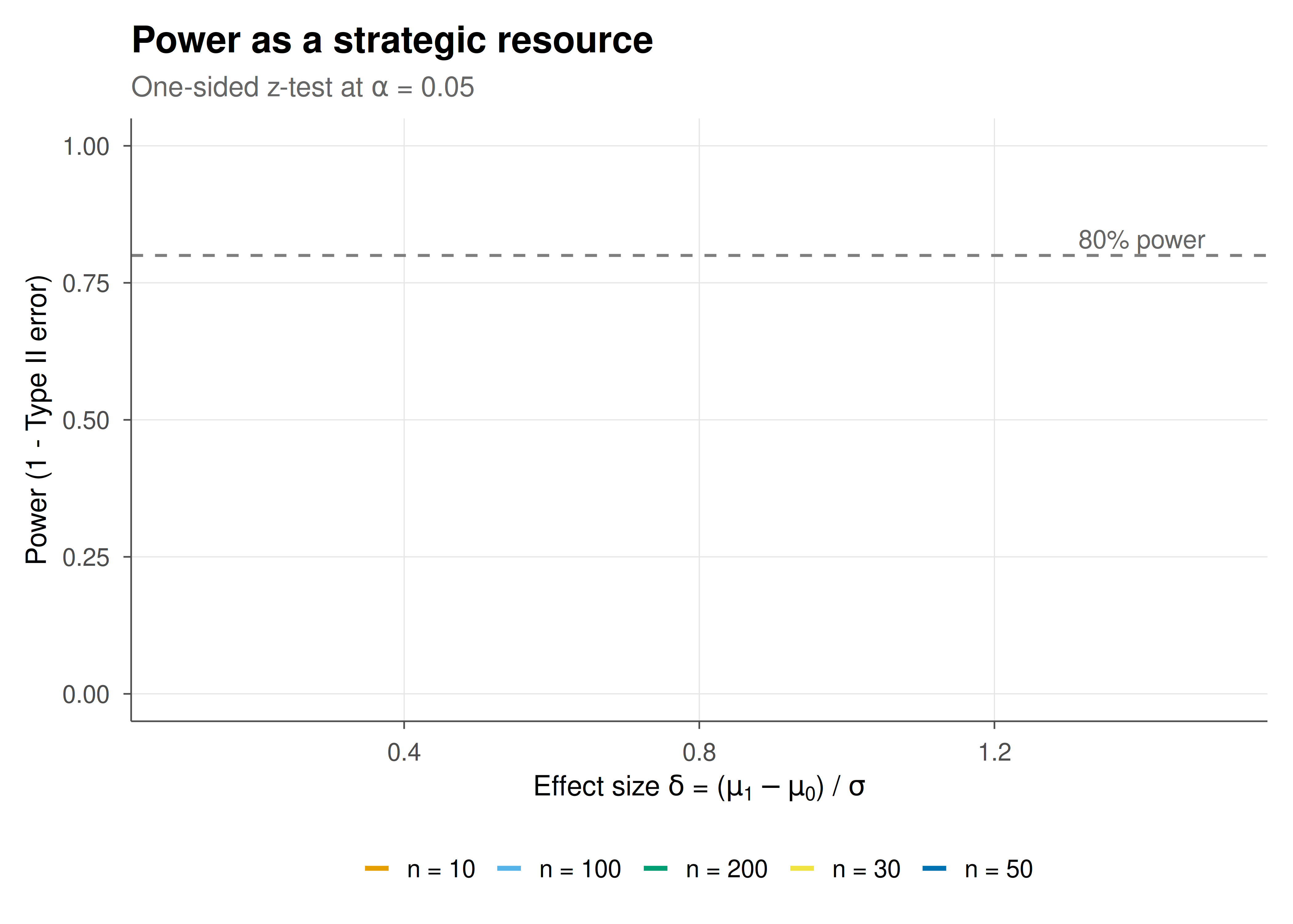
The power curves below map the statistician's strategic capacity: for each sample size, the curve traces the probability of correctly rejecting $H_0$ as a function of the true effect size. Larger samples shift the curve leftward, making even small effects detectable.
```{r}
#| label: fig-hypothesis-testing-static
#| fig-cap: "Figure 1. Power curves for the one-sided z-test at alpha = 0.05 across five sample sizes. The dashed horizontal line marks the conventional 80% power threshold. Larger samples enable detection of smaller effects. Okabe-Ito palette."
#| dev: [png, pdf]
#| fig-width: 7
#| fig-height: 5
#| dpi: 300
p_static <- ggplot(power_df, aes(x = delta, y = power, colour = n_label,
                                  text = paste0("Effect: ", round(delta, 2),
                                                "\nPower: ", round(power, 3),
                                                "\n", n_label))) +
  geom_line(linewidth = 0.9) +
  geom_hline(yintercept = 0.8, linetype = "dashed", colour = "grey50") +
  annotate("text", x = 1.4, y = 0.83, label = "80% power",
           colour = "grey40", size = 3.5) +
  scale_colour_manual(values = okabe_ito[1:5]) +
  labs(
    x = expression("Effect size " * delta * " = (" * mu[1] - mu[0] * ") / " * sigma),
    y = "Power (1 - Type II error)",
    colour = NULL,
    title = "Power as a strategic resource",
    subtitle = expression("One-sided z-test at " * alpha * " = 0.05")
  ) +
  coord_cartesian(ylim = c(0, 1)) +
  theme_publication()

save_pub_fig(p_static, "figures/hypothesis-testing-static")
p_static
```
## Interactive figure
Hover over the power curves to read off the exact power at any effect size and sample size combination. This is especially useful for sample-size planning, where the analyst needs to find the smallest $n$ that pushes the curve above the 80% threshold for a given expected effect.
```{r}
#| label: fig-hypothesis-testing-interactive
to_plotly_pub(p_static, tooltip = c("text"))
```
## Interpretation
The power curves make the strategic structure of hypothesis testing visually explicit. Nature's strongest move is to place the true effect size just above zero, where the statistician's test has almost no power regardless of sample size. The statistician's counter-strategy is to increase $n$, which compresses the null and alternative sampling distributions apart and shifts the power curve leftward. At $n = 200$, even a modest effect of $\delta = 0.3$ is detected with over 80% probability, whereas $n = 10$ requires an effect exceeding $\delta = 0.9$ to reach the same threshold.
This framing also illuminates the role of $\alpha$. The significance level is not an arbitrary convention but a constraint on the statistician's strategy set --- it bounds the probability of a false alarm. Relaxing $\alpha$ (raising it toward 0.10) uniformly increases power at the cost of more Type I errors, exactly as a player might trade defensive solidity for offensive capability. The Neyman--Pearson lemma guarantees that the likelihood ratio test extracts maximal power from the available $\alpha$ budget, making it the unique minimax-optimal response to Nature's choice.
A limitation of the simple normal model is that it assumes known variance. When $\sigma$ is estimated, the test statistic follows a $t$-distribution and the power formula requires noncentral $t$ calculations. This extension is straightforward but shifts the power curves slightly downward for small $n$.
## Extensions & related tutorials
The game-theoretic view extends naturally to composite hypotheses, where Nature chooses from a continuum $\Theta_1$ and the minimax test must guard against the least favourable distribution. Sequential testing (Wald's SPRT) adds a temporal dimension: the statistician dynamically decides when to stop sampling, turning the game into a stochastic optimal stopping problem. Multiple testing corrections (Bonferroni, Benjamini--Hochberg) can be interpreted as budget allocation across simultaneous games.
- [Building a game theory R package from scratch](../../r-package-development/building-game-theory-r-package/)
- [Modelling strategic interaction with VAR models](../../time-series-econometrics/strategic-interaction-var-models/)
- [Algorithmic fairness through the lens of game theory](../../ethics-applications/algorithmic-fairness-game-theory/)
## References
::: {#refs}
:::