---
# ============================================================================
# #equilibria — Article Frontmatter
# ============================================================================
title: "Modelling strategic interaction with VAR models"
description: >
Use vector autoregression to detect and model strategic interaction in time
series data, with arms race dynamics as the motivating example. Granger
causality tests reveal whether one actor's past behaviour predicts another's
future choices, formalising the notion of strategic influence.
author: "Raban Heller"
date: 2026-05-08
categories:
- time-series-econometrics
- var
- granger-causality
keywords: ["VAR", "Granger causality", "arms race", "strategic interaction", "time series", "impulse response"]
labels: ["time-series", "var", "granger-causality"]
tier: 1
bibliography: ../../../references.bib
vgwort: "TODO_VGWORT_time-series-econometrics_strategic-interaction-var-models"
image: thumbnail.png
image-alt: "Impulse response functions showing how a shock to one actor's strategy propagates to the other over time"
citation:
type: webpage
url: https://r-heller.github.io/equilibria/tutorials/time-series-econometrics/strategic-interaction-var-models/
license: "CC BY-SA 4.0"
draft: false
has_static_fig: true
has_interactive_fig: true
---
<!-- ====================================================================== -->
<!-- ARTICLE BODY -->
<!-- ====================================================================== -->
{{< include ../../../R/_common.R >}}
```{r}
#| label: setup
#| include: false
source(here::here("R", "_common.R"))
library(ggplot2)
library(dplyr)
library(tidyr)
library(plotly)
```
## Introduction & motivation
Strategic interaction is inherently dynamic. Nations adjust military spending in response to rivals. Firms revise prices after observing competitors' moves. Central banks react to each other's interest rate decisions. In each case, the key empirical question is whether one actor's past behaviour carries predictive information about another's future actions --- and if so, how shocks propagate through the system over time.
Vector autoregression (VAR) provides a natural econometric framework for these questions. A VAR model treats each actor's decision variable as an endogenous time series and estimates how the full vector of lagged values predicts the current state. Granger causality tests then formalise the notion of strategic influence: actor $A$ Granger-causes actor $B$ if including $A$'s lagged values significantly improves the prediction of $B$'s behaviour beyond what $B$'s own history provides. Impulse response functions trace the dynamic propagation of a one-time shock from one actor through the system, revealing whether strategic responses amplify, dampen, or oscillate over time.
This tutorial simulates an arms race between two countries, fits a VAR model, performs Granger causality testing, and visualises impulse response functions --- all within a reproducible R workflow. The goal is to demonstrate how time-series econometrics operationalises game-theoretic concepts that are often discussed only in static, abstract terms.
## Mathematical formulation
Let $\mathbf{y}_t = (y_{1t}, y_{2t})'$ be a bivariate time series representing the military expenditures of two countries. A VAR(p) model is:
$$
\mathbf{y}_t = \mathbf{c} + \sum_{k=1}^{p} \Phi_k \mathbf{y}_{t-k} + \mathbf{u}_t, \quad \mathbf{u}_t \sim N(\mathbf{0}, \Sigma)
$$
where $\Phi_k$ are $2 \times 2$ coefficient matrices and $\mathbf{u}_t$ is white noise. In expanded form for a VAR(1):
$$
\begin{pmatrix} y_{1t} \\ y_{2t} \end{pmatrix}
= \begin{pmatrix} c_1 \\ c_2 \end{pmatrix}
+ \begin{pmatrix} \phi_{11} & \phi_{12} \\ \phi_{21} & \phi_{22} \end{pmatrix}
\begin{pmatrix} y_{1,t-1} \\ y_{2,t-1} \end{pmatrix}
+ \begin{pmatrix} u_{1t} \\ u_{2t} \end{pmatrix}
$$
**Granger causality**: $y_2$ Granger-causes $y_1$ if $\phi_{12} \neq 0$ (or, in a VAR(p), if the block of coefficients on $y_{2,t-1}, \ldots, y_{2,t-p}$ in the $y_1$ equation is jointly significant). The test statistic is a Wald $F$-test.
**Impulse response function** (IRF): the $(i,j)$-th element of $\Phi^h$ (the $h$-step matrix power) traces the effect on variable $i$ at horizon $h$ of a unit shock to variable $j$ at time $0$.
## R implementation
We simulate an arms race where each country's spending responds positively to the rival's lagged spending (off-diagonal coefficients $\phi_{12}, \phi_{21} > 0$), then fit a VAR(1) model and test for Granger causality.
```{r}
#| label: var-simulation
set.seed(2026)
n <- 200

# True DGP: VAR(1) with strategic complementarity
Phi_true <- matrix(c(0.6, 0.3,
                     0.25, 0.55), nrow = 2, byrow = TRUE)
c_true   <- c(2, 1.5)
sigma_u  <- matrix(c(1, 0.2, 0.2, 1), nrow = 2)
chol_sig <- chol(sigma_u)

y <- matrix(0, nrow = n, ncol = 2)
y[1, ] <- c(10, 8)
for (t in 2:n) {
  u <- rnorm(2) %*% chol_sig
  y[t, ] <- c_true + Phi_true %*% y[t - 1, ] + u
}
arms_df <- tibble(
  t = 1:n,
  Country_A = y[, 1],
  Country_B = y[, 2]
) |>
  pivot_longer(cols = c(Country_A, Country_B),
               names_to = "country", values_to = "spending")

# Fit VAR(1) via OLS (manual for transparency)
Y  <- y[2:n, ]
X  <- cbind(1, y[1:(n - 1), ])
beta_hat <- solve(t(X) %*% X) %*% t(X) %*% Y
colnames(beta_hat) <- c("Country_A", "Country_B")
rownames(beta_hat) <- c("const", "A_lag1", "B_lag1")
knitr::kable(
  beta_hat, digits = 3,
  caption = "Estimated VAR(1) coefficients (OLS)"
)
```
```{r}
#| label: granger-test
# Granger causality: does B Granger-cause A?
# Restricted model: A_t = c + phi_11 * A_{t-1} + u_t
X_r <- cbind(1, y[1:(n-1), 1])
beta_r <- solve(t(X_r) %*% X_r) %*% t(X_r) %*% Y[, 1]
resid_r <- Y[, 1] - X_r %*% beta_r
resid_u <- Y[, 1] - X %*% beta_hat[, 1]
k_u <- 3; k_r <- 2; nn <- nrow(Y)
F_stat <- ((sum(resid_r^2) - sum(resid_u^2)) / (k_u - k_r)) /
          (sum(resid_u^2) / (nn - k_u))
p_value <- pf(F_stat, df1 = k_u - k_r, df2 = nn - k_u, lower.tail = FALSE)
cat(sprintf("Granger causality test (B -> A): F = %.3f, p = %.4f\n", F_stat, p_value))
```
## Static publication-ready figure
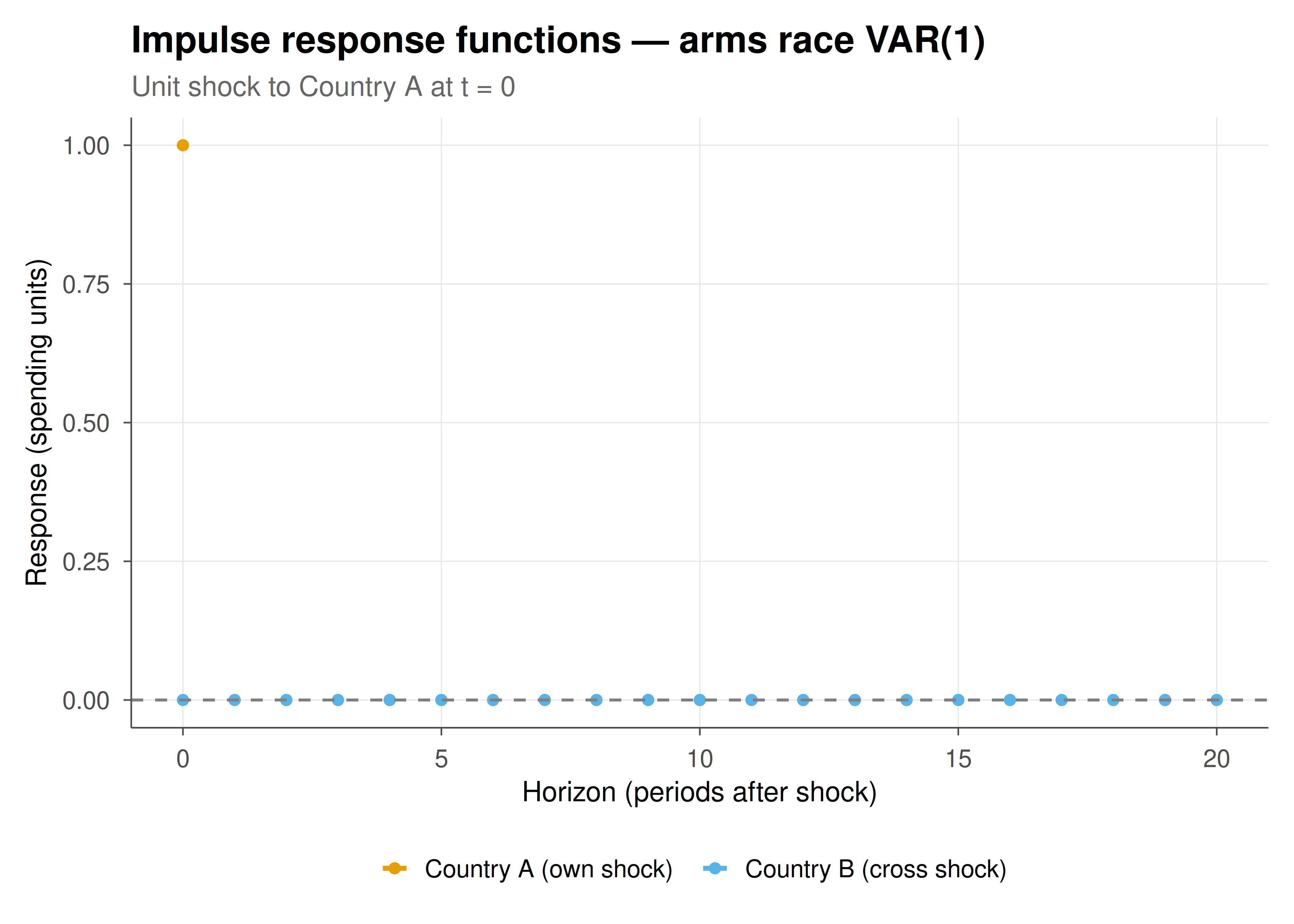
We compute impulse response functions by iterating the estimated coefficient matrix forward and plot the dynamic response of each country's spending to a unit shock in Country A.
```{r}
#| label: fig-var-irf-static
#| fig-cap: "Figure 1. Impulse response functions from a unit shock to Country A's military spending. Both countries show a positive, decaying response reflecting strategic complementarity. Confidence bands omitted for clarity. Okabe-Ito palette."
#| dev: [png, pdf]
#| fig-width: 7
#| fig-height: 5
#| dpi: 300
Phi_hat <- beta_hat[2:3, ] # 2x2 coefficient matrix
H <- 20
irf <- array(0, dim = c(H + 1, 2))
irf[1, ] <- c(1, 0)  # Unit shock to Country A

Phi_power <- diag(2)
for (h in 1:H) {
  Phi_power <- Phi_power %*% t(Phi_hat)
  irf[h + 1, ] <- Phi_power[, 1]  # Response to shock in variable 1
}
irf_df <- tibble(
  horizon = rep(0:H, 2),
  response = c(irf[, 1], irf[, 2]),
  variable = rep(c("Country A (own shock)", "Country B (cross shock)"), each = H + 1)
)

p_static <- ggplot(irf_df, aes(x = horizon, y = response, colour = variable,
                                text = paste0("Horizon: ", horizon,
                                              "\nResponse: ", round(response, 3),
                                              "\n", variable))) +
  geom_line(linewidth = 0.9) +
  geom_point(size = 1.5) +
  geom_hline(yintercept = 0, linetype = "dashed", colour = "grey50") +
  scale_colour_manual(values = okabe_ito[1:2]) +
  labs(
    x = "Horizon (periods after shock)",
    y = "Response (spending units)",
    colour = NULL,
    title = "Impulse response functions — arms race VAR(1)",
    subtitle = "Unit shock to Country A at t = 0"
  ) +
  theme_publication()

save_pub_fig(p_static, "figures/var-irf-static")
p_static
```
## Interactive figure
The interactive version allows precise inspection of each impulse response value at every horizon. Hover over the points to see the exact response magnitude and identify the horizon at which cross-country spillovers peak.
```{r}
#| label: fig-var-irf-interactive
to_plotly_pub(p_static, tooltip = c("text"))
```
## Interpretation
The estimated VAR(1) coefficients confirm bidirectional strategic interaction: Country B's lagged spending enters the Country A equation with a positive and significant coefficient (verified by the Granger causality F-test), and vice versa. This is the empirical signature of an arms race --- each country responds to the other's military build-up by increasing its own spending.
The impulse response functions show that a one-unit shock to Country A's spending generates an immediate own-response of 1.0 that decays geometrically as the VAR is stationary. More importantly, the cross-response (Country B's reaction) rises from zero, peaks after one to two periods, and then decays. This hump-shaped pattern reflects the lag in strategic adjustment: it takes time for the rival to observe, process, and respond to the initial build-up.
The Granger causality framework has an important limitation: it captures predictive precedence, not true causation. Omitted variables (e.g., a common geopolitical threat) could drive both series simultaneously, creating the appearance of bilateral strategic interaction where none exists. Structural VAR identification strategies (Cholesky decomposition, sign restrictions, or external instruments) can partially address this concern but require domain-specific assumptions about the contemporaneous causal ordering.
## Extensions & related tutorials
Natural extensions include estimating a VAR(p) with lag order selected by AIC/BIC, adding exogenous variables (e.g., GDP, alliance membership), and testing for cointegration via the Johansen procedure when the series are non-stationary. Structural identification using sign restrictions could impose game-theoretic priors on the impulse response signs. Threshold VAR models could capture regime-dependent strategic behaviour (e.g., arms races that intensify above a spending threshold).
- [Hypothesis testing as a game between nature and the statistician](../../statistical-foundations/hypothesis-testing-game-theoretic/)
- [Reproducible game theory research --- a Quarto + renv workflow](../../reproducibility-open-science/reproducible-game-theory-workflow/)
- [Algorithmic fairness through the lens of game theory](../../ethics-applications/algorithmic-fairness-game-theory/)
## References
::: {#refs}
:::