---
title: "Moran process in finite populations"
description: "Implement and analyze the Moran process for frequency-dependent selection in finite populations, computing fixation probabilities analytically and via simulation for 2-strategy evolutionary games."
author: "Raban Heller"
date: 2026-05-08
date-modified: 2026-05-08
categories:
- evolutionary-gt
- moran-process
- finite-populations
- stochastic-dynamics
keywords: ["Moran process", "fixation probability", "finite populations", "frequency-dependent selection", "stochastic evolution"]
labels: ["stochastic-dynamics", "finite-populations"]
tier: 1
bibliography: ../../../references.bib
vgwort: "TODO_VGWORT_evolutionary-gt_moran-process-finite-populations"
image: thumbnail.png
image-alt: "Fixation probability landscape for cooperators in the Prisoner's Dilemma under the Moran process as a function of population size and selection intensity"
citation:
type: webpage
url: https://r-heller.github.io/equilibria/tutorials/evolutionary-gt/moran-process-finite-populations/
license: "CC BY-SA 4.0"
draft: false
has_static_fig: true
has_interactive_fig: true
has_shiny_app: false
---
```{r}
#| label: setup
#| include: false
library(ggplot2)
library(dplyr)
library(tidyr)
library(plotly)
okabe_ito <- c("#E69F00", "#56B4E9", "#009E73", "#F0E442",
"#0072B2", "#D55E00", "#CC79A7", "#999999")
theme_publication <- function(base_size = 12) {
theme_minimal(base_size = base_size) +
theme(plot.title = element_text(size = base_size * 1.2, face = "bold"),
plot.subtitle = element_text(size = base_size * 0.9, color = "grey40"),
axis.line = element_line(color = "grey30", linewidth = 0.3),
panel.grid.minor = element_blank(), legend.position = "bottom",
plot.margin = margin(10, 10, 10, 10))
}
```
## Introduction & motivation
The replicator dynamics, which describes how strategy frequencies evolve in infinite populations under frequency-dependent selection, is a deterministic system: given initial conditions, the trajectory is completely determined. In real biological and social populations, however, population sizes are finite, and the dynamics are inherently stochastic. Random fluctuations — demographic stochasticity, or "drift" — can cause strategies to go extinct or fix even when selection favors the opposite outcome. The **Moran process**, introduced by Patrick Moran in 1958 and adapted to evolutionary game theory by @nowak_may_1992 and subsequent researchers, is the canonical stochastic model for evolutionary dynamics in finite populations. In each time step, one individual is selected for reproduction with probability proportional to fitness and one individual is selected for death uniformly at random. The offspring inherits the parent's strategy, so the population changes by at most one individual per step.
The Moran process is a birth-death Markov chain on the number of individuals playing each strategy. For a 2-strategy game with population size $N$, the state space is $\{0, 1, \ldots, N\}$ where state $k$ means $k$ individuals play strategy A and $N-k$ play strategy B. The absorbing states are $k=0$ (strategy A extinct) and $k=N$ (strategy A fixated). The central quantity of interest is the **fixation probability** $\rho_A$ — the probability that a single A-mutant introduced into a population of $N-1$ B-players eventually takes over the entire population. Under neutral drift (no selection), the fixation probability is simply $1/N$: every individual has an equal chance of being the ancestor of the entire future population. When selection is present, $\rho_A$ can be higher or lower than $1/N$ depending on whether strategy A is favored or disfavored.
The key insight from finite population analysis is that the predictions of infinite-population models (ESS, replicator dynamics) can fail dramatically when populations are small. A strategy that is an ESS and dominates under the replicator dynamics may nevertheless have a fixation probability below $1/N$ — meaning that selection actually *opposes* its spread in finite populations. Conversely, a strategy that would go extinct under the replicator dynamics can have $\rho > 1/N$ when $N$ is small enough, because drift overcomes weak counter-selection. This tutorial implements the Moran process for $2$-strategy games, computes fixation probabilities both analytically (using the exact formula for birth-death chains) and via Monte Carlo simulation, and compares the finite-population results with infinite-population predictions. We apply the analysis to the Prisoner's Dilemma with population sizes $N = 50$ to $200$, examining how population size and selection intensity jointly determine the fate of cooperation.
## Mathematical formulation
Consider a population of $N$ individuals playing a symmetric $2 \times 2$ game with payoff matrix:
$$
A = \begin{pmatrix} a & b \\ c & d \end{pmatrix}
$$
When there are $k$ individuals playing strategy A (cooperators) and $N-k$ playing strategy B (defectors), the expected payoffs are:
$$
f_A(k) = \frac{a(k-1) + b(N-k)}{N-1}, \quad f_B(k) = \frac{ck + d(N-k-1)}{N-1}
$$
Under frequency-dependent Moran process with **selection intensity** $w \in [0,1]$, fitness is:
$$
\phi_A(k) = 1 - w + w \cdot f_A(k), \quad \phi_B(k) = 1 - w + w \cdot f_B(k)
$$
The transition probabilities for the birth-death chain are:
$$
T^+(k) = \frac{k \cdot \phi_A(k)}{k \cdot \phi_A(k) + (N-k) \cdot \phi_B(k)} \cdot \frac{N-k}{N}
$$
$$
T^-(k) = \frac{(N-k) \cdot \phi_B(k)}{k \cdot \phi_A(k) + (N-k) \cdot \phi_B(k)} \cdot \frac{k}{N}
$$
The **fixation probability** of a single A-mutant is given by the exact formula for birth-death chains:
$$
\rho_A = \frac{1}{1 + \sum_{j=1}^{N-1} \prod_{k=1}^{j} \gamma_k}
$$
where $\gamma_k = T^-(k) / T^+(k)$ is the ratio of transition probabilities at state $k$.
Under **neutral drift** ($w = 0$), $\gamma_k = 1$ for all $k$, giving $\rho_A = 1/N$.
## R implementation
We implement the analytical fixation probability formula and a Monte Carlo simulator for the Moran process.
```{r}
#| label: moran-implementation
# Analytical fixation probability for 2-strategy Moran process
fixation_prob_analytical <- function(A, N, w = 0.01, initial_k = 1) {
  # A: 2x2 payoff matrix, N: population size, w: selection intensity
  a <- A[1,1]; b <- A[1,2]; c <- A[2,1]; d <- A[2,2]

  # Compute gamma_k = T^-(k) / T^+(k) for k = 1, ..., N-1
  gammas <- numeric(N - 1)
  for (k in 1:(N-1)) {
    f_A <- (a * (k - 1) + b * (N - k)) / (N - 1)
    f_B <- (c * k + d * (N - k - 1)) / (N - 1)
    phi_A <- 1 - w + w * f_A
    phi_B <- 1 - w + w * f_B
    gammas[k] <- phi_B / phi_A
  }

  # Fixation probability from state initial_k
  # rho_k = (1 + sum_{j=1}^{k-1} prod_{m=1}^{j} gamma_m) /
  #         (1 + sum_{j=1}^{N-1} prod_{m=1}^{j} gamma_m)

  cum_prod <- cumprod(gammas)
  denom <- 1 + sum(cum_prod)

  if (initial_k == 1) {
    rho <- 1 / denom
  } else {
    numer <- 1 + sum(cum_prod[1:(initial_k - 1)])
    rho <- numer / denom
  }

  return(rho)
}

# Monte Carlo simulation of Moran process
simulate_moran <- function(A, N, w = 0.01, initial_k = 1, n_runs = 5000) {
  a <- A[1,1]; b <- A[1,2]; c <- A[2,1]; d <- A[2,2]

  fixations <- 0

  for (run in 1:n_runs) {
    k <- initial_k
    while (k > 0 && k < N) {
      f_A <- (a * (k - 1) + b * (N - k)) / (N - 1)
      f_B <- (c * k + d * (N - k - 1)) / (N - 1)
      phi_A <- 1 - w + w * f_A
      phi_B <- 1 - w + w * f_B

      total_fitness <- k * phi_A + (N - k) * phi_B

      # Birth: proportional to fitness; Death: uniform
      # Prob increase = P(A born) * P(B dies) = (k*phi_A/total) * ((N-k)/N)
      prob_up <- (k * phi_A / total_fitness) * ((N - k) / N)
      prob_down <- ((N - k) * phi_B / total_fitness) * (k / N)

      r <- runif(1)
      if (r < prob_up) {
        k <- k + 1
      } else if (r < prob_up + prob_down) {
        k <- k - 1
      }
      # else: no change (same type born and dies)
    }
    if (k == N) fixations <- fixations + 1
  }

  return(fixations / n_runs)
}

# Prisoner's Dilemma payoff matrix
A_pd <- matrix(c(3, 0, 5, 1), nrow = 2, byrow = TRUE)
cat("Prisoner's Dilemma payoff matrix:\n")
cat(" C vs C =", A_pd[1,1], ", C vs D =", A_pd[1,2], "\n")
cat(" D vs C =", A_pd[2,1], ", D vs D =", A_pd[2,2], "\n\n")
# Compute fixation probabilities for various N
set.seed(42)
pop_sizes <- c(50, 75, 100, 150, 200)
w_sel <- 0.05

results <- data.frame(
  N = pop_sizes,
  neutral = 1 / pop_sizes,
  analytical = sapply(pop_sizes, function(n) fixation_prob_analytical(A_pd, n, w = w_sel)),
  simulated = sapply(pop_sizes, function(n) simulate_moran(A_pd, n, w = w_sel, n_runs = 3000))
)

cat("Fixation probability of a single cooperator (w =", w_sel, "):\n")
print(results, digits = 5)
cat("\nRatio rho_C / (1/N) — values < 1 mean selection opposes cooperation:\n")
cat(round(results$analytical / results$neutral, 4), "\n")
```
Now we compute fixation probabilities across a range of selection intensities.
```{r}
#| label: selection-intensity-sweep
# Sweep over selection intensity
N_fixed <- 100
w_values <- seq(0, 0.2, by = 0.005)

fixation_sweep <- data.frame(
  w = w_values,
  rho_C = sapply(w_values, function(w) fixation_prob_analytical(A_pd, N_fixed, w)),
  rho_D = sapply(w_values, function(w) {
    # Fixation of defector = fixation of strategy 2 in transposed game
    A_transposed <- matrix(c(A_pd[2,2], A_pd[2,1], A_pd[1,2], A_pd[1,1]),
                           nrow = 2, byrow = TRUE)
    fixation_prob_analytical(A_transposed, N_fixed, w)
  })
)

fixation_sweep$neutral <- 1 / N_fixed

cat("Fixation probabilities at N =", N_fixed, "for selected w values:\n")
fixation_sweep |>
  filter(w %in% c(0, 0.01, 0.05, 0.1, 0.2)) |>
  print(digits = 5)
```
## Static publication-ready figure
We visualize the fixation probability landscape showing how population size and selection intensity jointly determine whether cooperation can spread.
```{r}
#| label: fig-moran-fixation
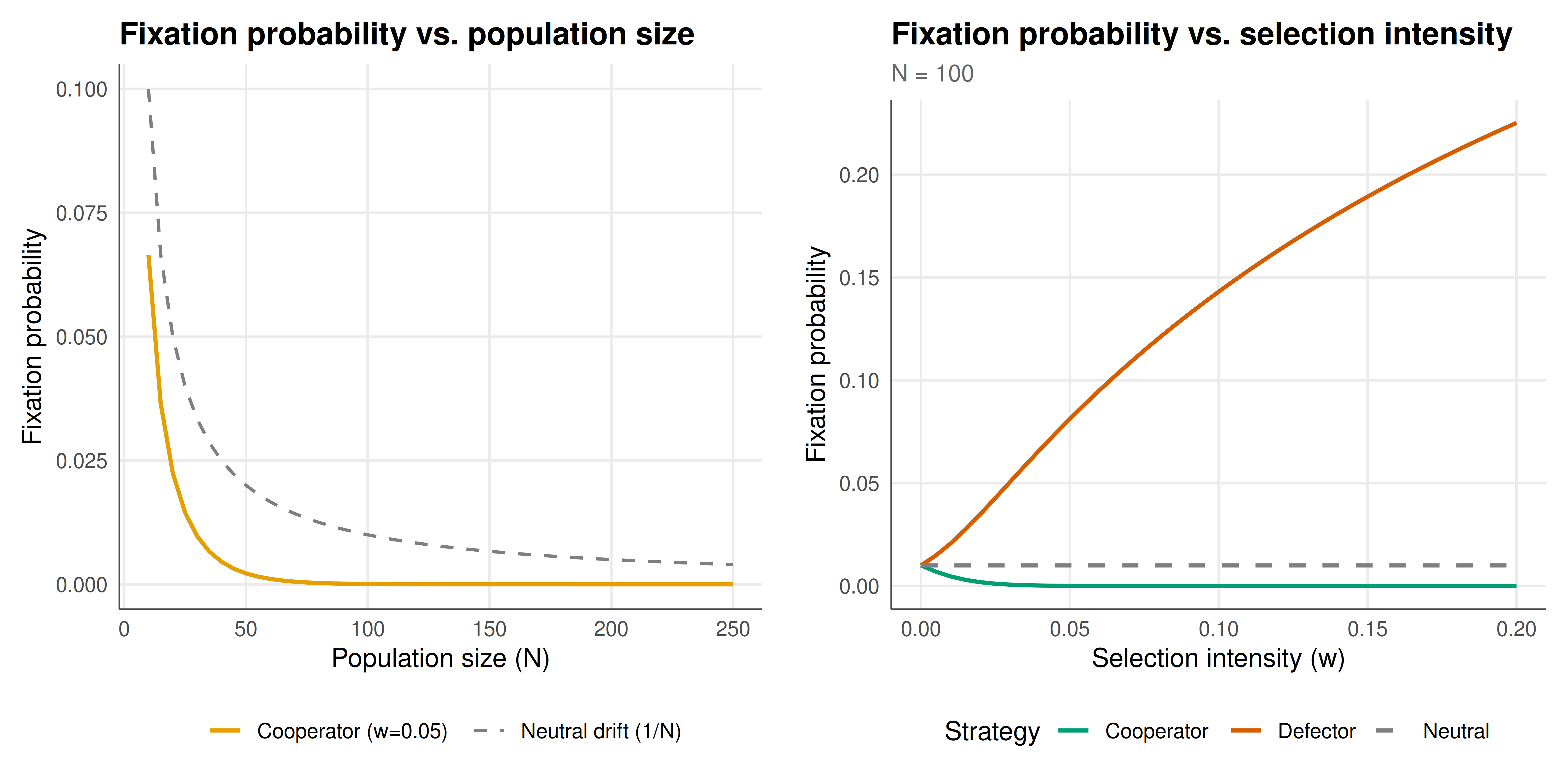
#| fig-cap: "Figure 1. Fixation probability of a single cooperator in the Prisoner's Dilemma under the Moran process. Left panel: fixation probability versus population size at selection intensity w = 0.05 (orange), compared to neutral drift 1/N (dashed grey). Right panel: fixation probability versus selection intensity at N = 100. In both panels, cooperator fixation is below the neutral baseline, confirming that selection opposes cooperation in the PD — but the effect is modest for weak selection."
#| dev: [png, pdf]
#| fig-width: 10
#| fig-height: 5
#| dpi: 300
# Panel 1: Fixation vs population size
N_range <- seq(10, 250, by = 5)
fix_vs_N <- data.frame(
  N = N_range,
  rho_analytical = sapply(N_range, function(n) fixation_prob_analytical(A_pd, n, w = 0.05)),
  neutral = 1 / N_range
)

p1 <- ggplot(fix_vs_N) +
  geom_line(aes(x = N, y = neutral, color = "Neutral drift (1/N)"),
            linetype = "dashed", linewidth = 0.7) +
  geom_line(aes(x = N, y = rho_analytical, color = "Cooperator (w=0.05)"),
            linewidth = 0.9) +
  scale_color_manual(values = c("Neutral drift (1/N)" = "grey50",
                                 "Cooperator (w=0.05)" = okabe_ito[1]),
                     name = "") +
  labs(title = "Fixation probability vs. population size",
       x = "Population size (N)", y = "Fixation probability") +
  theme_publication() +
  theme(legend.position = "bottom")

# Panel 2: Fixation vs selection intensity
fix_long <- fixation_sweep |>
  select(w, Cooperator = rho_C, Defector = rho_D, Neutral = neutral) |>
  pivot_longer(-w, names_to = "Strategy", values_to = "Fixation")

p2 <- ggplot(fix_long, aes(x = w, y = Fixation, color = Strategy)) +
  geom_line(aes(linetype = Strategy), linewidth = 0.9) +
  scale_color_manual(values = c("Cooperator" = okabe_ito[3],
                                 "Defector" = okabe_ito[6],
                                 "Neutral" = "grey50")) +
  scale_linetype_manual(values = c("Cooperator" = "solid",
                                    "Defector" = "solid",
                                    "Neutral" = "dashed")) +
  labs(title = "Fixation probability vs. selection intensity",
       subtitle = paste0("N = ", N_fixed),
       x = "Selection intensity (w)", y = "Fixation probability") +
  theme_publication() +
  theme(legend.position = "bottom")

# Combine panels using patchwork-style approach with base grid
gridExtra::grid.arrange(p1, p2, ncol = 2)
```
## Interactive figure
The interactive figure shows individual Moran process trajectories alongside the analytical fixation probability, allowing exploration of the stochastic dynamics.
```{r}
#| label: fig-moran-interactive
# Simulate a few individual Moran trajectories for visualization
set.seed(123)
simulate_moran_trajectory <- function(A, N, w = 0.05, initial_k = 1, max_steps = 50000) {
  a <- A[1,1]; b <- A[1,2]; c <- A[2,1]; d <- A[2,2]
  trajectory <- integer(max_steps + 1)
  trajectory[1] <- initial_k
  k <- initial_k

  for (step in 1:max_steps) {
    if (k == 0 || k == N) break
    f_A <- (a * (k - 1) + b * (N - k)) / (N - 1)
    f_B <- (c * k + d * (N - k - 1)) / (N - 1)
    phi_A <- 1 - w + w * f_A
    phi_B <- 1 - w + w * f_B
    total_fitness <- k * phi_A + (N - k) * phi_B

    prob_up <- (k * phi_A / total_fitness) * ((N - k) / N)
    prob_down <- ((N - k) * phi_B / total_fitness) * (k / N)

    r <- runif(1)
    if (r < prob_up) k <- k + 1
    else if (r < prob_up + prob_down) k <- k - 1
    trajectory[step + 1] <- k
  }

  # Trim to actual length
  end_step <- min(which(trajectory == 0 | trajectory == N), max_steps + 1)
  data.frame(step = 0:(end_step - 1), k = trajectory[1:end_step])
}

N_traj <- 50
n_trajectories <- 8

traj_list <- lapply(1:n_trajectories, function(i) {
  tr <- simulate_moran_trajectory(A_pd, N_traj, w = 0.05, initial_k = 1)
  tr$run <- paste0("Run ", i)
  tr$outcome <- ifelse(tr$k[nrow(tr)] == N_traj, "Fixation", "Extinction")
  tr$text <- sprintf("Step: %d\nCooperators: %d/%d\nRun: %s",
                      tr$step, tr$k, N_traj, tr$run)
  tr
})

traj_df <- bind_rows(traj_list)

p_traj <- ggplot(traj_df, aes(x = step, y = k / N_traj, color = run, text = text)) +
  geom_line(linewidth = 0.4, alpha = 0.8) +
  geom_hline(yintercept = 1 / N_traj, linetype = "dotted", color = "grey60") +
  scale_color_manual(values = rep(okabe_ito, length.out = n_trajectories)) +
  labs(
    title = paste0("Moran process trajectories (N=", N_traj, ", PD, w=0.05)"),
    subtitle = "Each line is one realization starting from 1 cooperator",
    x = "Time step",
    y = "Cooperator frequency"
  ) +
  theme_publication() +
  theme(legend.position = "none")

ggplotly(p_traj, tooltip = "text") |>
  config(displaylogo = FALSE,
         modeBarButtonsToRemove = c("select2d", "lasso2d"))
```
## Interpretation
The Moran process analysis reveals several important insights that complement and extend the predictions of infinite-population evolutionary game theory. First, for the Prisoner's Dilemma, the fixation probability of a single cooperator is consistently below the neutral benchmark of $1/N$, confirming that selection opposes cooperation — as expected, since Defect dominates Cooperate and is the unique ESS. However, the magnitude of this selection effect depends critically on both the population size $N$ and the selection intensity $w$. Under weak selection ($w \ll 1$), the fixation probability is only slightly below $1/N$, meaning that drift can still occasionally carry cooperation to fixation despite the selective disadvantage. This "weak selection" regime is biologically plausible and has been the focus of much recent theoretical work.
Second, the relationship between population size and fixation probability is non-trivial. While larger populations reduce the absolute fixation probability (since $1/N$ shrinks), they also amplify the relative effect of selection: the ratio $\rho_C / (1/N)$ decreases with $N$, meaning that selection against cooperation becomes relatively stronger in larger populations. This is a general feature of the Moran process: larger populations are more "deterministic" and more faithfully track the infinite-population predictions. In the limit $N \to \infty$, the Moran process converges to the replicator dynamics (after appropriate time rescaling), and the fixation probability of a disfavored strategy goes to zero.
Third, the individual trajectory visualization reveals the dramatic stochasticity of the process when $N$ is moderate. Most runs starting from a single cooperator end in rapid extinction (the absorbing state $k = 0$), but occasional runs show the cooperator count drifting upward before eventually returning to zero. The rare event of fixation requires the cooperator to survive an extended initial period where it constitutes a tiny minority — a feat that becomes exponentially unlikely as selection intensity increases or population size grows. This stochastic perspective is essential for understanding how cooperation can persist in nature despite its apparent evolutionary disadvantage in one-shot interactions.
## Extensions & related tutorials
- [Evolutionarily stable strategies (ESS)](../evolutionarily-stable-strategies/) — the infinite-population stability concept that the Moran process refines and sometimes contradicts.
- [Replicator dynamics for Rock-Paper-Scissors](../replicator-dynamics-rps/) — the deterministic infinite-population dynamics that the Moran process approximates as $N \to \infty$.
- [Nash equilibrium in mixed strategies](../../foundations/nash-equilibrium-mixed/) — the static equilibrium concept underlying the evolutionary dynamics.
- [Folk theorem with perfect monitoring](../../foundations/folk-theorem-perfect-monitoring/) — an alternative route to cooperation through repeated interaction rather than evolutionary dynamics.
## References
::: {#refs}
:::