---
title: "Replicator-mutator dynamics — evolution with mutation"
description: "Extend the standard replicator equation with a mutation matrix Q, implement the ODE system using deSolve in R, and show how mutation stabilises the interior equilibrium of Rock-Paper-Scissors."
author: "Raban Heller"
date: 2026-05-08
date-modified: 2026-05-08
categories:
- evolutionary-gt
- replicator-mutator
- mutation
- rock-paper-scissors
keywords: ["replicator-mutator dynamics", "mutation matrix", "evolutionary game theory", "deSolve", "Rock-Paper-Scissors"]
labels: ["evolutionary-dynamics", "mutation"]
tier: 1
bibliography: ../../../references.bib
vgwort: "TODO_VGWORT_evolutionary-gt_replicator-mutator-dynamics"
image: thumbnail.png
image-alt: "Time series comparing replicator dynamics with and without mutation in Rock-Paper-Scissors, showing how mutation stabilises cyclic orbits"
citation:
type: webpage
url: https://r-heller.github.io/equilibria/tutorials/evolutionary-gt/replicator-mutator-dynamics/
license: "CC BY-SA 4.0"
draft: false
has_static_fig: true
has_interactive_fig: true
has_shiny_app: false
---
```{r}
#| label: setup
#| include: false
library(ggplot2)
library(dplyr)
library(tidyr)
library(plotly)
okabe_ito <- c("#E69F00", "#56B4E9", "#009E73", "#F0E442",
"#0072B2", "#D55E00", "#CC79A7", "#999999")
theme_publication <- function(base_size = 12) {
theme_minimal(base_size = base_size) +
theme(plot.title = element_text(size = base_size * 1.2, face = "bold"),
plot.subtitle = element_text(size = base_size * 0.9, color = "grey40"),
axis.line = element_line(color = "grey30", linewidth = 0.3),
panel.grid.minor = element_blank(), legend.position = "bottom",
plot.margin = margin(10, 10, 10, 10))
}
```
## Introduction & motivation
The replicator equation is the workhorse of evolutionary game theory. It captures the core Darwinian idea that strategies producing above-average fitness grow in frequency, while those performing below average decline. For many games of biological and economic interest, the replicator dynamics provides an elegant deterministic description of how populations evolve over time. Yet standard replicator dynamics rests on a critical simplifying assumption: offspring inherit their parent's strategy perfectly, with no errors, no experimentation, and no random exploration of the strategy space. In biological reality, mutation is ubiquitous. In economic and social contexts, agents occasionally experiment with new strategies, make mistakes, or imitate imperfectly. The replicator-mutator equation extends the classical framework by introducing a mutation matrix $Q$ that governs the probability that offspring of a parent playing strategy $j$ instead adopt strategy $i$. This seemingly modest extension has profound consequences for the qualitative behaviour of the dynamical system.
The replicator-mutator equation was developed in the context of quasispecies theory by Eigen and Schuster in the late 1970s, originally to model the evolution of self-replicating RNA molecules. In their framework, the mutation matrix captures copying errors during molecular replication, and the interplay between selection and mutation determines which "quasispecies" — clouds of closely related sequences — dominate the population. The same mathematical structure later appeared independently in evolutionary game theory, where it models populations of agents who occasionally switch strategies through trembling-hand errors, experimentation, or imperfect social learning. The replicator-mutator equation has since become a central tool in theoretical biology, linguistics (modelling language evolution), and behavioural economics (modelling bounded rationality in learning dynamics).
The game we use throughout this tutorial is Rock-Paper-Scissors (RPS). Under pure replicator dynamics, RPS exhibits neutrally stable cyclic orbits around the interior Nash equilibrium at $(1/3, 1/3, 1/3)$. The system possesses a conserved quantity $V = x_R \cdot x_P \cdot x_S$, which means orbits neither converge to the equilibrium nor diverge to the boundary — they cycle perpetually. This structural property is fragile: it relies on the exact cancellation of forces in the skew-symmetric payoff matrix. Any perturbation — whether from stochastic noise, spatial structure, or mutation — will generically break the conservation law and change the qualitative behaviour of the system. Mutation, in particular, introduces a restoring force that pulls trajectories away from the boundary and toward the interior. The key question we investigate is: does mutation cause orbits to spiral inward (stabilising the equilibrium) or outward (destabilising it)?
In this tutorial, we derive the replicator-mutator equation, implement it as an ODE system in R using the `deSolve` package, and simulate the dynamics for RPS with symmetric uniform mutation. We show that even a small mutation rate converts the neutrally stable centre of pure replicator dynamics into an asymptotically stable spiral — orbits converge to the interior equilibrium. We then explore how the convergence rate depends on the mutation rate $\mu$ and visualise the bifurcation that occurs as $\mu$ varies from zero to large values. The tutorial builds directly on the companion article on pure replicator dynamics for RPS and provides the foundation for understanding more complex evolutionary processes where mutation, selection, and drift interact.
## Mathematical formulation
Let $n$ be the number of strategies and let $x = (x_1, \ldots, x_n)$ denote the population state on the $(n-1)$-simplex $\Delta^{n-1}$. The payoff matrix is $A \in \mathbb{R}^{n \times n}$ where $a_{ij}$ is the payoff to strategy $i$ against strategy $j$. The fitness of strategy $i$ is:
$$
f_i(x) = (Ax)_i = \sum_{j=1}^{n} a_{ij} x_j
$$
The average population fitness is $\bar{f}(x) = x^\top A x = \sum_i x_i f_i(x)$.
The mutation matrix $Q = (q_{ij})$ is a row-stochastic matrix where $q_{ij}$ is the probability that an offspring of a parent playing strategy $j$ adopts strategy $i$. Note the convention: $q_{ij}$ gives the flow from $j$ to $i$, so each column of $Q$ sums to one.
The **replicator-mutator equation** is:
$$
\dot{x}_i = \sum_{j=1}^{n} x_j f_j(x) \, q_{ij} - x_i \bar{f}(x)
$$
The first term accounts for all the ways strategy $i$ can be produced: a parent of any type $j$, present at frequency $x_j$ with fitness $f_j$, mutates to produce an $i$-offspring with probability $q_{ij}$. The second term is the dilution due to population growth at the mean rate $\bar{f}$.
For symmetric uniform mutation with rate $\mu \in [0, 1]$, the mutation matrix is:
$$
q_{ij} = \begin{cases} 1 - \mu & \text{if } i = j \\ \frac{\mu}{n-1} & \text{if } i \neq j \end{cases}
$$
When $\mu = 0$, we recover the standard replicator equation. When $\mu = 1$, all offspring are uniformly random regardless of the parent's type, and selection is completely overwhelmed by mutation.
For the RPS payoff matrix:
$$
A = \begin{pmatrix} 0 & -1 & 1 \\ 1 & 0 & -1 \\ -1 & 1 & 0 \end{pmatrix}
$$
the interior equilibrium $x^* = (1/3, 1/3, 1/3)$ remains a fixed point of the replicator-mutator equation for any symmetric $Q$ (by symmetry of both $A$ and $Q$). A linear stability analysis around $x^*$ reveals that for $\mu > 0$ the eigenvalues of the Jacobian acquire negative real parts, so $x^*$ becomes an asymptotically stable spiral. The imaginary parts of the eigenvalues generate oscillatory approach, but the real parts ensure convergence — the mutation breaks the conservation law of pure replicator dynamics.
## R implementation
We implement the replicator-mutator ODE system and compare trajectories with and without mutation.
```{r}
#| label: replicator-mutator-ode
library(deSolve)

set.seed(42)

# RPS payoff matrix
A_rps <- matrix(c(0, -1, 1,
                   1,  0, -1,
                  -1,  1, 0), nrow = 3, byrow = TRUE)

# Mutation matrix: symmetric uniform mutation with rate mu
make_Q <- function(n, mu) {
  Q <- matrix(mu / (n - 1), nrow = n, ncol = n)
  diag(Q) <- 1 - mu
  Q
}

# Replicator-mutator ODE
replicator_mutator <- function(t, state, parms) {
  x <- state
  A <- parms$A
  Q <- parms$Q
  fitness <- as.numeric(A %*% x)
  avg_fitness <- sum(x * fitness)
  # dx_i/dt = sum_j x_j f_j Q_ij - x_i * f_bar
  dxdt <- as.numeric(Q %*% (x * fitness)) - x * avg_fitness
  list(dxdt)
}

# Simulation parameters
times <- seq(0, 60, by = 0.05)
x0 <- c(0.6, 0.2, 0.2)
mu_values <- c(0, 0.01, 0.05, 0.15)

results <- lapply(mu_values, function(mu) {
  Q <- make_Q(3, mu)
  sol <- ode(y = x0, times = times, func = replicator_mutator,
             parms = list(A = A_rps, Q = Q), method = "rk4")
  df <- as.data.frame(sol)
  names(df) <- c("time", "Rock", "Paper", "Scissors")
  df$mu <- mu
  df$label <- paste0("mu = ", mu)
  df$V <- df$Rock * df$Paper * df$Scissors
  df
})

traj_df <- bind_rows(results)

cat("Final state at t = 60 for each mutation rate:\n")
traj_df |>
  group_by(label) |>
  summarise(
    Rock = round(last(Rock), 4),
    Paper = round(last(Paper), 4),
    Scissors = round(last(Scissors), 4),
    V_final = round(last(V), 6),
    .groups = "drop"
  ) |>
  print()
cat("\nDeviation from equilibrium (1/3, 1/3, 1/3) at t = 60:\n")
traj_df |>
  group_by(label) |>
  summarise(
    max_dev = round(max(abs(last(Rock) - 1/3),
                        abs(last(Paper) - 1/3),
                        abs(last(Scissors) - 1/3)), 6),
    .groups = "drop"
  ) |>
  print()
```
```{r}
#| label: bifurcation-analysis
# Measure convergence: distance from equilibrium at t = 60
mu_grid <- seq(0, 0.3, by = 0.005)
convergence_data <- lapply(mu_grid, function(mu) {
  Q <- make_Q(3, mu)
  sol <- ode(y = x0, times = times, func = replicator_mutator,
             parms = list(A = A_rps, Q = Q), method = "rk4")
  df <- as.data.frame(sol)
  names(df) <- c("time", "Rock", "Paper", "Scissors")
  final <- tail(df, 1)
  dev <- sqrt((final$Rock - 1/3)^2 + (final$Paper - 1/3)^2 +
              (final$Scissors - 1/3)^2)
  data.frame(mu = mu, distance = dev)
})

bif_df <- bind_rows(convergence_data)

cat("Bifurcation data (selected mutation rates):\n")
bif_df |>
  filter(mu %in% c(0, 0.01, 0.05, 0.1, 0.2, 0.3)) |>
  print()
```
## Static publication-ready figure
```{r}
#| label: fig-replicator-mutator-comparison
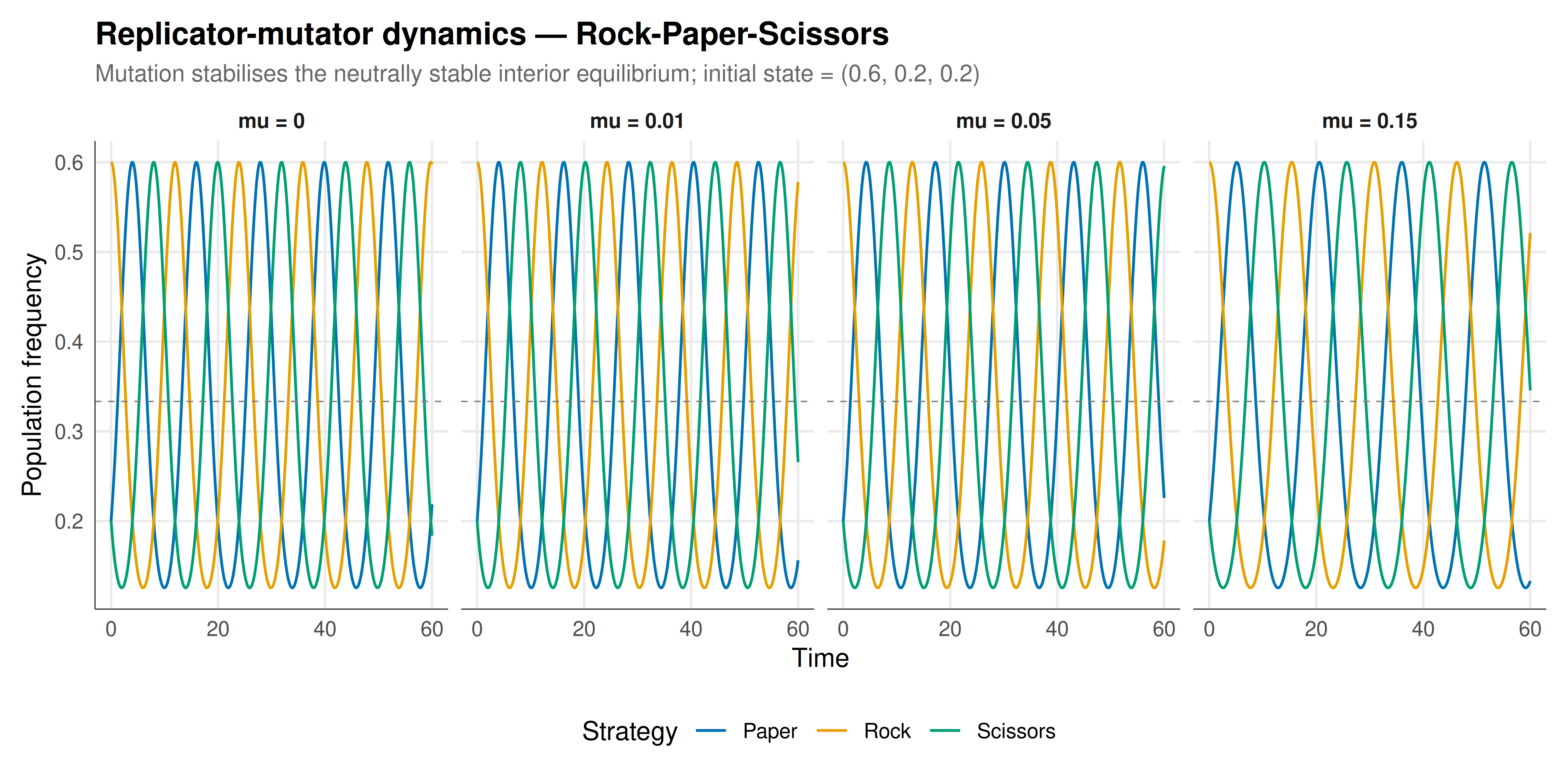
#| fig-cap: "Figure 1. Replicator-mutator dynamics for Rock-Paper-Scissors with varying mutation rates. Without mutation (mu = 0), strategies cycle indefinitely. With increasing mutation, orbits spiral inward to the equilibrium (1/3, 1/3, 1/3). The dashed grey line marks the equilibrium frequency. Okabe-Ito palette."
#| dev: [png, pdf]
#| fig-width: 10
#| fig-height: 5
#| dpi: 300
traj_long <- traj_df |>
  filter(mu %in% c(0, 0.01, 0.05, 0.15)) |>
  select(time, Rock, Paper, Scissors, label) |>
  pivot_longer(c(Rock, Paper, Scissors),
               names_to = "Strategy", values_to = "Frequency") |>
  mutate(label = factor(label, levels = paste0("mu = ", c(0, 0.01, 0.05, 0.15))))

p_static <- ggplot(traj_long, aes(x = time, y = Frequency, color = Strategy)) +
  geom_line(linewidth = 0.6) +
  geom_hline(yintercept = 1/3, linetype = "dashed", color = "grey50",
             linewidth = 0.3) +
  facet_wrap(~label, nrow = 1) +
  scale_color_manual(values = c(Rock = okabe_ito[1], Paper = okabe_ito[5],
                                 Scissors = okabe_ito[3])) +
  labs(
    title = "Replicator-mutator dynamics — Rock-Paper-Scissors",
    subtitle = "Mutation stabilises the neutrally stable interior equilibrium; initial state = (0.6, 0.2, 0.2)",
    x = "Time", y = "Population frequency"
  ) +
  theme_publication() +
  theme(strip.text = element_text(face = "bold"))

p_static
```
## Interactive figure
```{r}
#| label: fig-bifurcation-interactive
bif_df <- bif_df |>
  mutate(text = sprintf("Mutation rate: %.3f\nDistance from eq.: %.5f",
                         mu, distance))

p_bif <- ggplot(bif_df, aes(x = mu, y = distance, text = text)) +
  geom_line(color = okabe_ito[5], linewidth = 0.8) +
  geom_point(color = okabe_ito[5], size = 1.5) +
  geom_vline(xintercept = 0, linetype = "dashed", color = okabe_ito[6]) +
  labs(
    title = "Bifurcation: distance from equilibrium at t = 60",
    subtitle = "mu = 0 gives persistent cycling; any mu > 0 yields convergence",
    x = "Mutation rate (mu)",
    y = "Euclidean distance from (1/3, 1/3, 1/3)"
  ) +
  theme_publication()

ggplotly(p_bif, tooltip = "text") |>
  config(displaylogo = FALSE,
         modeBarButtonsToRemove = c("select2d", "lasso2d"))
```
## Interpretation
The simulations reveal a sharp qualitative difference between pure replicator dynamics and the replicator-mutator equation. Under the standard replicator dynamics ($\mu = 0$), the Rock-Paper-Scissors system produces closed cyclic orbits around the interior equilibrium $(1/3, 1/3, 1/3)$, as guaranteed by the conserved quantity $V = x_R x_P x_S$. The orbit amplitude and period depend on the initial condition, but no trajectory ever converges to the equilibrium — the system is neutrally stable, a degenerate case poised between stability and instability. This behaviour, while mathematically elegant, is structurally fragile: any perturbation to the dynamics can tip the system one way or the other.
Mutation provides exactly such a perturbation, and the direction it tips is always toward stability. Even a tiny mutation rate $\mu = 0.01$ converts the neutrally stable centre into an asymptotically stable spiral. The oscillations persist — the imaginary parts of the Jacobian eigenvalues at the equilibrium remain nonzero — but they decay exponentially, with the population state spiralling inward to $(1/3, 1/3, 1/3)$. At higher mutation rates ($\mu = 0.05$ and $\mu = 0.15$), convergence is faster and the oscillatory transient is shorter. The bifurcation plot confirms that the transition is discontinuous in a qualitative sense: at $\mu = 0$ the system cycles forever (distance from equilibrium remains positive and constant), while for any $\mu > 0$ the distance decays to zero. This is a supercritical Hopf-like bifurcation in reverse — as mutation increases from zero, a centre becomes a stable focus.
The mechanism behind this stabilisation is intuitive. In pure replicator dynamics, a strategy that becomes rare faces no intrinsic restoring force — its growth rate depends only on its relative fitness, which in RPS creates a perpetual chase. Mutation introduces a baseline flow of individuals into every strategy regardless of fitness. When Rock is rare, some Paper and Scissors players "mutate" to Rock, providing a demographic floor. When Rock is common, some Rock players mutate away, providing a ceiling. This mean-reverting force acts like friction in a physical system: it dissipates the "energy" that sustains the conservative orbits and brings the system to rest at the equilibrium.
The bifurcation analysis further reveals that the convergence rate (measured by the distance from equilibrium at a fixed time horizon) increases monotonically with $\mu$, but with diminishing returns. There is a trade-off: higher mutation accelerates convergence but also means the population spends more time exploring suboptimal strategies. In biological contexts, this corresponds to the mutation-selection balance — too much mutation degrades adaptation, while too little fails to explore the fitness landscape. The intermediate regime, where mutation is strong enough to stabilise dynamics but weak enough that selection still matters, is the most biologically relevant. This tutorial demonstrates how to systematically explore this trade-off using numerical ODE solutions and bifurcation diagrams, techniques that generalise immediately to games with more strategies and more complex mutation structures.
## Extensions & related tutorials
- [Replicator dynamics for Rock-Paper-Scissors](../replicator-dynamics-rps/) — the baseline model without mutation, showing conserved cyclic orbits.
- [Moran process in finite populations](../moran-process-finite-populations/) — stochastic evolutionary dynamics where genetic drift interacts with selection and mutation.
- [Evolutionarily stable strategies (ESS)](../evolutionarily-stable-strategies/) — understanding when equilibria resist invasion, with and without mutation.
- [Hawk-Dove and the war of attrition](../hawk-dove-war-of-attrition/) — applying replicator-mutator dynamics to asymmetric contests.
- [Spatial evolutionary games](../../simulations/spatial-prisoners-dilemma-nowak-may/) — how spatial structure provides an alternative stabilisation mechanism.
## References
::: {#refs}
:::