---
title: "Hawk-Dove and the war of attrition — escalation in evolutionary games"
description: "Model the continuous-time war of attrition as an extension of the Hawk-Dove game in R, derive the mixed ESS with exponential waiting times, and visualise how resource value and fighting costs shape escalation behaviour."
author: "Raban Heller"
date: 2026-05-08
date-modified: 2026-05-08
categories:
- evolutionary-gt
- hawk-dove
- war-of-attrition
- escalation
keywords: ["war of attrition", "Hawk-Dove", "escalation", "ESS", "evolutionary game theory", "fighting costs"]
labels: ["evolutionary-dynamics", "conflict-models"]
tier: 1
bibliography: ../../../references.bib
vgwort: "TODO_VGWORT_evolutionary-gt_hawk-dove-war-of-attrition"
image: thumbnail.png
image-alt: "Expected contest duration and payoffs in the war of attrition as functions of resource value"
citation:
type: webpage
url: https://r-heller.github.io/equilibria/tutorials/evolutionary-gt/hawk-dove-war-of-attrition/
license: "CC BY-SA 4.0"
draft: false
has_static_fig: true
has_interactive_fig: true
has_shiny_app: false
---
```{r}
#| label: setup
#| include: false
library(ggplot2)
library(dplyr)
library(tidyr)
library(plotly)
okabe_ito <- c("#E69F00", "#56B4E9", "#009E73", "#F0E442",
"#0072B2", "#D55E00", "#CC79A7", "#999999")
theme_publication <- function(base_size = 12) {
theme_minimal(base_size = base_size) +
theme(plot.title = element_text(size = base_size * 1.2, face = "bold"),
plot.subtitle = element_text(size = base_size * 0.9, color = "grey40"),
axis.line = element_line(color = "grey30", linewidth = 0.3),
panel.grid.minor = element_blank(), legend.position = "bottom",
plot.margin = margin(10, 10, 10, 10))
}
```
## Introduction & motivation
The **war of attrition**, introduced by Maynard Smith in 1974, extends the discrete Hawk-Dove game into continuous time: two animals contest a resource by waiting, each accumulating costs per unit time, and the first to quit loses the resource. Unlike the discrete game where Hawk and Dove are fixed strategies, the war of attrition asks: how long should a contestant persist? The remarkable answer is that the unique symmetric Nash equilibrium (and ESS) involves **randomised persistence** — each player chooses a waiting time from an exponential distribution with rate $c/V$, where $V$ is the resource value and $c$ is the cost per unit time. This means that on average, total fighting costs equal the resource value — the contest is exactly as wasteful as the resource is valuable. The war of attrition model applies far beyond biology: patent races (firms invest in R&D hoping competitors will drop out), lobbying contests (interest groups spend to outlast opponents), political standoffs (governments wait out each other in negotiations), and online auctions with sunk bidding costs (all-pay auctions). The model reveals a deep tension in competitive escalation: rational agents cannot commit to fighting "just long enough" because any deterministic strategy is exploitable. Only by randomising — making your persistence unpredictable — can you prevent your opponent from timing their quit to beat you. This tutorial derives the ESS for the war of attrition, simulates contests between exponential-strategy players, compares outcomes with the discrete Hawk-Dove game, and visualises how the value-to-cost ratio shapes escalation dynamics and contest wastage.
## Mathematical formulation
**Discrete Hawk-Dove** payoff matrix (value $V$, cost $C$, $C > V$):
$$\begin{pmatrix} (V-C)/2 & V \\ 0 & V/2 \end{pmatrix}$$
Mixed ESS: $p^* = V/C$ (probability of playing Hawk).
**War of attrition**: Two players choose persistence times $t_1, t_2 \geq 0$. The player who persists longer wins the resource $V$; both pay cost $c \cdot \min(t_1, t_2)$. Payoffs:
$$u_i(t_i, t_j) = \begin{cases} V - c \cdot t_j & \text{if } t_i > t_j \\ -c \cdot t_i & \text{if } t_i < t_j \\ V/2 - c \cdot t_i & \text{if } t_i = t_j \end{cases}$$
**Symmetric ESS**: Each player draws $t_i$ from an exponential distribution:
$$F(t) = 1 - e^{-t \cdot c/V}, \quad f(t) = \frac{c}{V} e^{-t \cdot c/V}$$
Expected payoff at ESS: $E[u_i] = 0$ (all surplus dissipated by contest costs).
## R implementation
```{r}
#| label: war-of-attrition
set.seed(42)

# === War of attrition parameters ===
V <- 10   # resource value
c_cost <- 2  # cost per unit time

# ESS: exponential with rate c/V
rate_ess <- c_cost / V
cat(sprintf("=== War of Attrition ===\n"))
cat(sprintf("Resource value V = %.0f, cost rate c = %.0f\n", V, c_cost))
cat(sprintf("ESS: Exp(rate = c/V = %.2f), mean persistence = V/c = %.1f\n",
            rate_ess, V/c_cost))
# === Simulate contests ===
n_contests <- 20000
t1 <- rexp(n_contests, rate = rate_ess)
t2 <- rexp(n_contests, rate = rate_ess)

winner <- ifelse(t1 > t2, 1, ifelse(t2 > t1, 2, 0))
contest_duration <- pmin(t1, t2)
payoff1 <- ifelse(winner == 1, V - c_cost * t2, -c_cost * pmin(t1, t2))
payoff2 <- ifelse(winner == 2, V - c_cost * t1, -c_cost * pmin(t1, t2))

cat(sprintf("\n--- Simulation (%d contests) ---\n", n_contests))
cat(sprintf("Mean contest duration: %.3f (theory: V/(2c) = %.3f)\n",
            mean(contest_duration), V / (2 * c_cost)))
cat(sprintf("Mean total cost: %.3f (theory: V = %.1f)\n",
            mean(c_cost * (t1 + ifelse(winner == 1, t2, ifelse(winner == 2, t1, t1)))),
            V))
cat(sprintf("Mean payoff (each player): %.3f (theory: 0)\n", mean(payoff1)))
cat(sprintf("P(player 1 wins): %.3f (theory: 0.5)\n", mean(winner == 1)))
# === Comparison: discrete Hawk-Dove ===
C_hd <- 15  # fighting cost (C > V for interesting dynamics)
p_hawk <- V / C_hd
cat(sprintf("\n--- Discrete Hawk-Dove (C=%.0f) ---\n", C_hd))
cat(sprintf("Mixed ESS: p(Hawk) = V/C = %.3f\n", p_hawk))
cat(sprintf("Expected payoff at ESS: %.3f\n", 0)) # E[u] = 0 at interior ESS in HD
# === Value-to-cost ratio analysis ===
vc_ratios <- seq(0.5, 20, by = 0.5)
woa_stats <- sapply(vc_ratios, function(vc) {
  rate <- 1 / vc  # c/V with c=1
  t_a <- rexp(5000, rate)
  t_b <- rexp(5000, rate)
  dur <- pmin(t_a, t_b)
  c(mean_duration = mean(dur), mean_total_cost = mean(dur) * 2 * 1,
    waste_ratio = mean(dur) * 2 / vc)
})

cat(sprintf("\nWaste ratio (total cost / V) ≈ 1.0 across all V/c ratios: confirmed = %.2f\n",
            mean(woa_stats[3,])))
```
## Static publication-ready figure
```{r}
#| label: fig-war-of-attrition
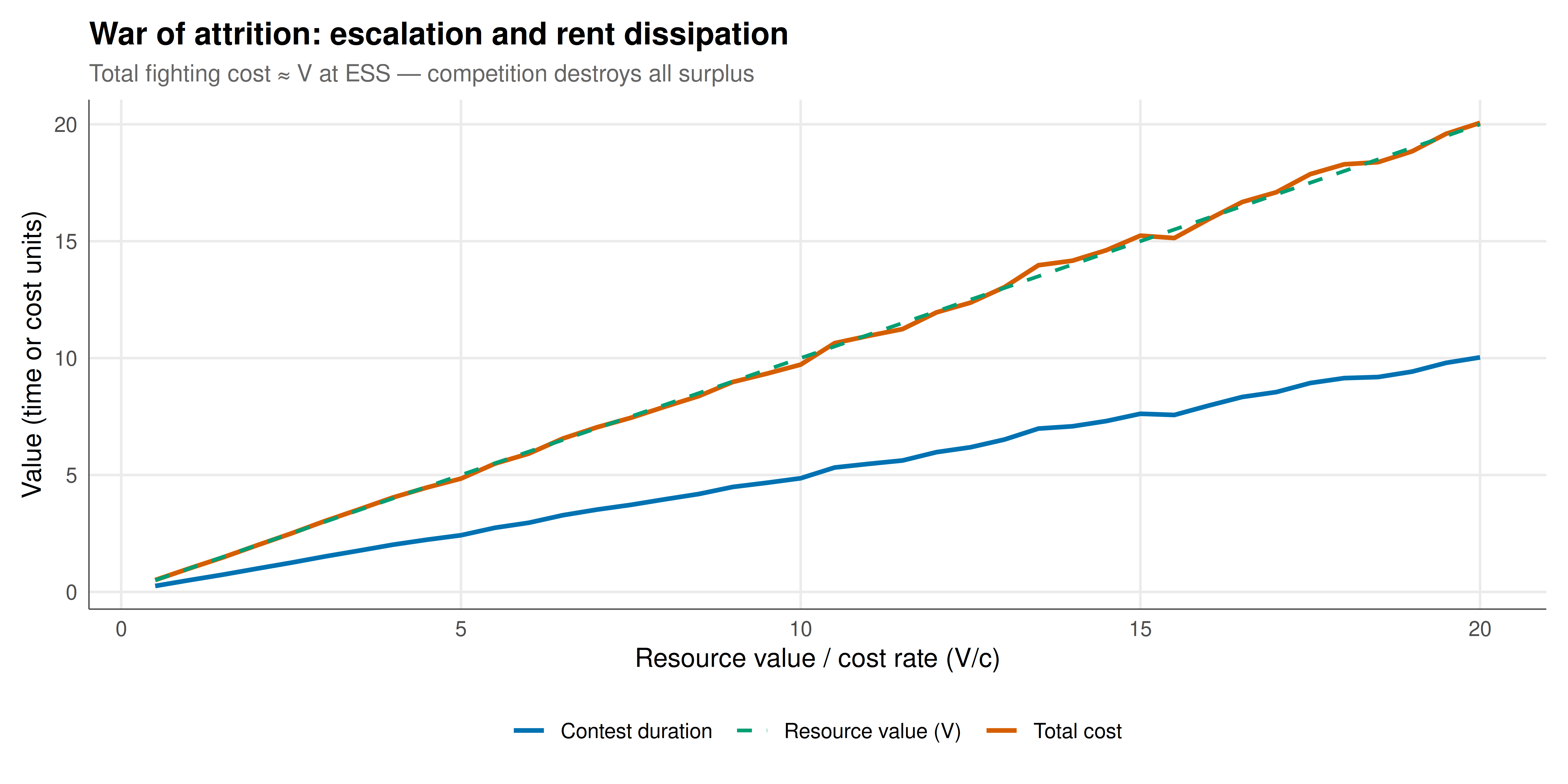
#| fig-cap: "Figure 1. War of attrition outcomes across different resource value-to-cost ratios. Left: mean contest duration increases linearly with V/c — more valuable resources provoke longer fights. Right: the total cost of fighting (both players combined) equals the resource value on average, confirming complete rent dissipation at the ESS. This is the fundamental insight of the war of attrition: in equilibrium, competition destroys exactly as much surplus as the prize is worth. Okabe-Ito palette."
#| dev: [png, pdf]
#| fig-width: 10
#| fig-height: 5
#| dpi: 300
woa_df <- tibble(
  vc_ratio = vc_ratios,
  mean_duration = woa_stats[1, ],
  mean_total_cost = woa_stats[2, ]
)

p1_data <- woa_df |> select(vc_ratio, mean_duration) |>
  mutate(panel = "Mean contest duration")
p2_data <- woa_df |> select(vc_ratio, value = mean_total_cost) |>
  mutate(panel = "Total fighting cost vs resource value")
p2_data$resource_value <- p2_data$vc_ratio  # V when c=1

ggplot(woa_df) +
  geom_line(aes(x = vc_ratio, y = mean_duration, color = "Contest duration"),
            linewidth = 1) +
  geom_line(aes(x = vc_ratio, y = mean_total_cost, color = "Total cost"),
            linewidth = 1) +
  geom_line(aes(x = vc_ratio, y = vc_ratio, color = "Resource value (V)"),
            linewidth = 0.8, linetype = "dashed") +
  scale_color_manual(values = c("Contest duration" = okabe_ito[5],
                                 "Total cost" = okabe_ito[6],
                                 "Resource value (V)" = okabe_ito[3]),
                      name = NULL) +
  labs(title = "War of attrition: escalation and rent dissipation",
       subtitle = "Total fighting cost ≈ V at ESS — competition destroys all surplus",
       x = "Resource value / cost rate (V/c)", y = "Value (time or cost units)") +
  theme_publication()
```
## Interactive figure
```{r}
#| label: fig-woa-contest-distribution
# Distribution of contest durations for different V/c ratios
dur_data <- lapply(c(1, 3, 5, 10), function(vc) {
  rate <- 1 / vc
  durations <- rexp(5000, rate)
  tibble(vc_ratio = paste0("V/c = ", vc), duration = durations)
}) |> bind_rows()

# Empirical CDF
dur_summary <- dur_data |>
  group_by(vc_ratio) |>
  arrange(duration) |>
  mutate(
    ecdf = row_number() / n(),
    text = paste0(vc_ratio, "\nDuration: ", round(duration, 2),
                  "\nP(contest ≤ t): ", round(ecdf, 3))
  )

p_dur <- ggplot(dur_summary, aes(x = duration, y = ecdf, color = vc_ratio, text = text)) +
  geom_step(linewidth = 0.7) +
  scale_color_manual(values = okabe_ito[c(1, 3, 5, 6)], name = "Value/Cost") +
  labs(title = "Contest duration distributions — war of attrition",
       subtitle = "Higher V/c → heavier tail (more prolonged contests)",
       x = "Contest duration (time units)", y = "Cumulative probability") +
  coord_cartesian(xlim = c(0, 30)) +
  theme_publication()

ggplotly(p_dur, tooltip = "text") |>
  config(displaylogo = FALSE, modeBarButtonsToRemove = c("select2d", "lasso2d"))
```
## Interpretation
The war of attrition reveals one of the most counterintuitive results in game theory: in equilibrium, rational agents waste resources in exact proportion to what they're fighting over. This "complete rent dissipation" result means that from a social welfare perspective, the contest produces zero net surplus — the expected cost of fighting exactly equals the prize. The mechanism is subtle: any player who systematically quits early can be exploited by a patient opponent, and any player who systematically persists too long pays excessive costs. Only by randomising persistence (exponential distribution) can a player make themselves unexploitable. The exponential distribution is the unique memoryless distribution — at every moment during the contest, your remaining willingness to wait is independent of how long you've already waited, which means your opponent gains no information from observing that you haven't quit yet. This memorylessness property is what makes the ESS unexploitable. The connection to the discrete Hawk-Dove game is precise: the war of attrition is the continuous-time limit where Hawk = "persist forever" and Dove = "quit immediately" are replaced by a continuum of persistence times. The same V/C trade-off governs both: when resources are valuable relative to fighting costs, contests are more aggressive (longer in WoA, more Hawks in HD). Applications to economic contests are direct: in patent races, firms invest up to the patent's expected value; in lobbying, interest groups collectively spend amounts comparable to the rents they seek; in all-pay auctions, total bids converge to the item's value. Understanding this dynamic is essential for designing institutions that reduce wasteful competition — caps on campaign spending, arbitration mechanisms, or property rights that avoid the contest altogether.
## Extensions & related tutorials
- [Chicken / Hawk-Dove game](../../classical-games/chicken-hawk-dove/) — the discrete foundation.
- [Evolutionarily stable strategies](../evolutionarily-stable-strategies/) — ESS theory for the discrete version.
- [Replicator dynamics for RPS](../replicator-dynamics-rps/) — evolutionary dynamics in another context.
- [First-price auction equilibrium](../../auction-theory-deep-dive/first-price-sealed-bid/) — all-pay auction connections.
- [Colonel Blotto game](../../classical-games/colonel-blotto/) — another resource allocation contest.
## References
::: {#refs}
:::