---
title: "The Colonel Blotto game — resource allocation across battlefields"
description: "Analyse the Colonel Blotto game in R, exploring optimal resource allocation across multiple battlefields, mixed-strategy equilibria, and applications to political campaigns and military strategy."
author: "Raban Heller"
date: 2026-05-08
date-modified: 2026-05-08
categories:
- classical-games
- blotto
- resource-allocation
- mixed-strategies
keywords: ["Colonel Blotto", "resource allocation", "battlefield game", "mixed strategy", "zero-sum game", "political campaigns"]
labels: ["canonical-games", "zero-sum-games"]
tier: 1
bibliography: ../../../references.bib
vgwort: "TODO_VGWORT_classical-games_colonel-blotto"
image: thumbnail.png
image-alt: "Ternary heatmap showing Colonel Blotto allocation strategies across three battlefields"
citation:
type: webpage
url: https://r-heller.github.io/equilibria/tutorials/classical-games/colonel-blotto/
license: "CC BY-SA 4.0"
draft: false
has_static_fig: true
has_interactive_fig: true
has_shiny_app: false
---
```{r}
#| label: setup
#| include: false
library(ggplot2)
library(dplyr)
library(tidyr)
library(plotly)
okabe_ito <- c("#E69F00", "#56B4E9", "#009E73", "#F0E442",
"#0072B2", "#D55E00", "#CC79A7", "#999999")
theme_publication <- function(base_size = 12) {
theme_minimal(base_size = base_size) +
theme(
plot.title = element_text(size = base_size * 1.2, face = "bold"),
plot.subtitle = element_text(size = base_size * 0.9, color = "grey40"),
axis.line = element_line(color = "grey30", linewidth = 0.3),
panel.grid.minor = element_blank(),
legend.position = "bottom",
plot.margin = margin(10, 10, 10, 10)
)
}
```
## Introduction & motivation
The Colonel Blotto game, introduced by Emile Borel in 1921 and systematically analysed by Gross and Wagner (1950), is one of the oldest and most elegant models in game theory. Two colonels (players) each command a fixed number of troops, which they must simultaneously allocate across $K$ battlefields. A player wins a battlefield if they commit strictly more troops to it than their opponent; the player who wins the majority of battlefields wins the engagement. This deceptively simple setup produces remarkably rich strategic behaviour because the constraint that total resources are fixed creates interdependencies: committing more troops to one battlefield necessarily means committing fewer to another. Unlike many textbook games with small strategy spaces, the Blotto game features a continuous (or high-dimensional discrete) strategy space, and its equilibria are generically in **mixed strategies** -- pure-strategy Nash equilibria do not exist when resources are equal and the number of battlefields is at least three.
The Colonel Blotto game has experienced a renaissance in political science and economics because it provides a natural model for electoral competition with multiple districts. A political campaign has a fixed budget (money, candidate time, advertising) that must be allocated across states or districts; the candidate who wins the majority of districts wins the election. The Blotto framework explains why campaigns sometimes adopt surprising strategies -- concentrating resources in unexpected places -- and why the weaker player (fewer total resources) may still have a positive probability of winning through clever asymmetric allocation. Myerson (1993) showed that the game has counterintuitive properties in the limit of many battlefields: the advantage of having more resources diminishes, and even a modestly outgunned player can win with high probability if they adopt the right distribution over allocations. Roberson (2006) provided the full characterization of mixed-strategy equilibria for the continuous version, showing that equilibrium strategies involve jointly uniform marginals across battlefields. In this tutorial, we implement the discrete Blotto game for $K = 3$ battlefields, enumerate the feasible allocations, compute win rates through simulation of mixed strategies, and visualize the results in a ternary-style heatmap. The analysis reveals why diversified allocation strategies tend to outperform concentrated ones, and how asymmetric resources dramatically reshape the strategic landscape.
## Mathematical formulation
Two players each have $N_1$ and $N_2$ troops respectively, allocated across $K$ battlefields. An **allocation** for player $i$ is a vector $(x_1, x_2, \ldots, x_K)$ with $x_j \geq 0$ and $\sum_{j=1}^K x_j = N_i$.
Player $i$ wins battlefield $j$ if $x_j^i > x_j^{-i}$ (ties can be split or counted as half-wins). The **payoff** is the number of battlefields won:
$$
u_i(\mathbf{x}^i, \mathbf{x}^{-i}) = \sum_{j=1}^{K} \mathbf{1}\{x_j^i > x_j^{-i}\} + \frac{1}{2}\sum_{j=1}^{K} \mathbf{1}\{x_j^i = x_j^{-i}\}
$$
For the symmetric game ($N_1 = N_2 = N$) with $K = 3$, the number of feasible integer allocations is $\binom{N+K-1}{K-1} = \binom{N+2}{2}$. No **pure-strategy Nash equilibrium** exists: for any fixed allocation by one player, the other can always find a winning counter-allocation. To see this, suppose player 1 plays $(a, b, c)$ with $a + b + c = N$. Player 2 can play $(b+1, c+1, a - 2)$ (when feasible), winning two out of three battlefields with minimal reallocation. This best-response cycling means the equilibrium must be in mixed strategies.
For the continuous version on $[0, N]^K$, Roberson (2006) showed that the unique equilibrium for $K = 3$ and equal budgets involves each player randomizing over allocations such that the **marginal distribution on each battlefield is uniform** on $[0, 2N/3]$. The key insight is that concentrating resources is punished -- a uniform spread across battlefields is the hardest distribution to exploit.
For **asymmetric budgets** ($N_1 > N_2$), the stronger player wins with higher probability but cannot guarantee winning all battlefields. The weaker player's optimal strategy involves randomizing to occasionally concentrate forces, creating the possibility of upset victories.
## R implementation
```{r}
#| label: blotto-analysis
# Generate all integer allocations of N troops across K battlefields
blotto_allocations <- function(N, K) {
  if (K == 1) return(matrix(N, ncol = 1))
  allocs <- list()
  # Recursive generation for K battlefields
  generate <- function(remaining, fields_left, current) {
    if (fields_left == 1) {
      allocs[[length(allocs) + 1]] <<- c(current, remaining)
      return()
    }
    for (x in 0:remaining) {
      generate(remaining - x, fields_left - 1, c(current, x))
    }
  }
  generate(N, K, c())
  do.call(rbind, allocs)
}

# Compute Blotto outcome: battlefields won by player 1
blotto_outcome <- function(alloc1, alloc2) {
  wins <- sum(alloc1 > alloc2)
  ties <- sum(alloc1 == alloc2)
  wins + 0.5 * ties
}

# Enumerate allocations for K=3
N <- 10
K <- 3
allocs <- blotto_allocations(N, K)
n_allocs <- nrow(allocs)

cat(sprintf("=== Colonel Blotto: N=%d troops, K=%d battlefields ===\n", N, K))
cat(sprintf("Number of feasible allocations: %d\n", n_allocs))
cat(sprintf("Expected: C(%d+%d-1, %d-1) = C(%d, %d) = %d\n",
            N, K, K, N+K-1, K-1, choose(N+K-1, K-1)))
# Compute full payoff matrix (row player wins)
payoff_matrix <- matrix(0, nrow = n_allocs, ncol = n_allocs)
for (i in 1:n_allocs) {
  for (j in 1:n_allocs) {
    payoff_matrix[i, j] <- blotto_outcome(allocs[i, ], allocs[j, ])
  }
}

# Win rate of each allocation against uniform opponent
win_rates <- rowMeans(payoff_matrix > K/2)
tie_rates <- rowMeans(payoff_matrix == K/2)

best_idx <- which.max(win_rates)
worst_idx <- which.min(win_rates)

cat(sprintf("\nBest allocation (vs uniform): (%s) — win rate = %.1f%%\n",
            paste(allocs[best_idx, ], collapse = ", "), 100 * win_rates[best_idx]))
cat(sprintf("Worst allocation (vs uniform): (%s) — win rate = %.1f%%\n",
            paste(allocs[worst_idx, ], collapse = ", "), 100 * win_rates[worst_idx]))
# Concentration measure: max troops on any single battlefield
concentration <- apply(allocs, 1, max)
cat("\n=== Win rate by concentration (max troops on one battlefield) ===\n")
conc_summary <- tibble(
  concentration = concentration,
  win_rate = win_rates
) |>
  group_by(concentration) |>
  summarise(
    mean_win = mean(win_rate),
    n_strategies = n(),
    .groups = "drop"
  )
for (i in 1:nrow(conc_summary)) {
  cat(sprintf("  Max = %2d: mean win rate = %.1f%% (%d strategies)\n",
              conc_summary$concentration[i],
              100 * conc_summary$mean_win[i],
              conc_summary$n_strategies[i]))
}
# Asymmetric game: N1=12 vs N2=10
cat("\n=== Asymmetric game: 12 vs 10 troops ===\n")
allocs_12 <- blotto_allocations(12, 3)
allocs_10 <- blotto_allocations(10, 3)

asym_payoff <- matrix(0, nrow = nrow(allocs_12), ncol = nrow(allocs_10))
for (i in 1:nrow(allocs_12)) {
  for (j in 1:nrow(allocs_10)) {
    asym_payoff[i, j] <- blotto_outcome(allocs_12[i, ], allocs_10[j, ])
  }
}

# Win rate of player 1 (12 troops) vs uniform player 2 (10 troops)
p1_wins <- mean(asym_payoff > K/2)
cat(sprintf("Player 1 (12 troops) wins %.1f%% of matchups vs Player 2 (10 troops)\n", 100 * p1_wins))
```
## Static publication-ready figure
```{r}
#| label: fig-blotto-heatmap
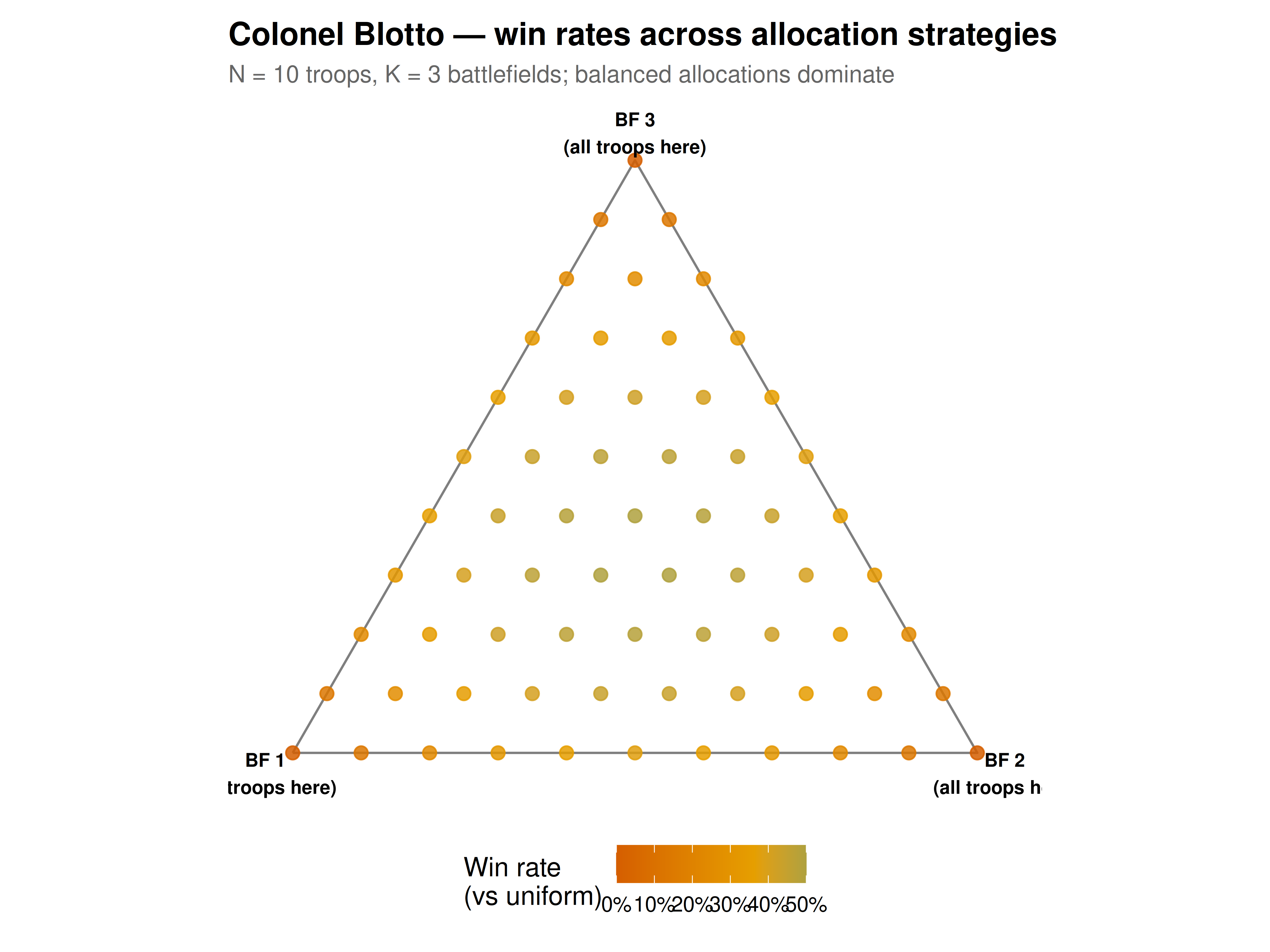
#| fig-cap: "Figure 1. Win rates for Colonel Blotto allocations (N = 10 troops, K = 3 battlefields) against a uniformly random opponent. Each point represents an allocation (x, y, z) with x + y + z = 10, projected onto 2D simplex coordinates. Balanced allocations near the centre achieve higher win rates than extreme allocations at the edges. The colour gradient shows win probability, with brighter colours indicating superior strategies. Okabe-Ito inspired palette."
#| dev: [png, pdf]
#| fig-width: 8
#| fig-height: 6
#| dpi: 300
# Project 3D simplex to 2D coordinates for ternary-style plot
simplex_to_2d <- function(a, b, c) {
  total <- a + b + c
  x <- 0.5 * (2 * b + c) / total
  y <- (sqrt(3) / 2) * c / total
  data.frame(x = x, y = y)
}

plot_data <- simplex_to_2d(allocs[, 1], allocs[, 2], allocs[, 3]) |>
  mutate(
    bf1 = allocs[, 1],
    bf2 = allocs[, 2],
    bf3 = allocs[, 3],
    win_rate = win_rates,
    concentration = concentration
  )

# Triangle boundary
tri_x <- c(0, 1, 0.5, 0)
tri_y <- c(0, 0, sqrt(3)/2, 0)

p_ternary <- ggplot(plot_data, aes(x = x, y = y)) +
  # Triangle boundary
  annotate("path", x = tri_x, y = tri_y, color = "grey50", linewidth = 0.5) +
  # Points coloured by win rate
  geom_point(aes(color = win_rate), size = 2.5, alpha = 0.85) +
  scale_color_gradient2(
    low = okabe_ito[6], mid = okabe_ito[1], high = okabe_ito[3],
    midpoint = median(win_rates),
    name = "Win rate\n(vs uniform)",
    labels = scales::percent_format(accuracy = 1)
  ) +
  # Vertex labels
  annotate("text", x = -0.04, y = -0.03, label = "BF 1\n(all troops here)",
           size = 3, fontface = "bold", hjust = 0.5) +
  annotate("text", x = 1.04, y = -0.03, label = "BF 2\n(all troops here)",
           size = 3, fontface = "bold", hjust = 0.5) +
  annotate("text", x = 0.5, y = sqrt(3)/2 + 0.04, label = "BF 3\n(all troops here)",
           size = 3, fontface = "bold", hjust = 0.5) +
  labs(
    title = "Colonel Blotto — win rates across allocation strategies",
    subtitle = sprintf("N = %d troops, K = %d battlefields; balanced allocations dominate", N, K)
  ) +
  coord_fixed() +
  theme_publication() +
  theme(
    axis.text = element_blank(),
    axis.title = element_blank(),
    axis.line = element_blank(),
    panel.grid.major = element_blank()
  )

p_ternary
```
## Interactive figure
```{r}
#| label: fig-blotto-interactive
# Interactive scatter: win rate vs concentration with allocation details
interactive_data <- plot_data |>
  mutate(
    label = sprintf("(%d, %d, %d)", bf1, bf2, bf3),
    text = paste0("Allocation: (", bf1, ", ", bf2, ", ", bf3, ")",
                  "\nWin rate: ", round(100 * win_rate, 1), "%",
                  "\nMax on one BF: ", concentration)
  )

p_conc <- ggplot(interactive_data, aes(x = concentration, y = win_rate, text = text)) +
  geom_jitter(aes(color = factor(concentration)), width = 0.15,
              size = 2, alpha = 0.7) +
  geom_smooth(method = "loess", se = TRUE, color = "grey30",
              linewidth = 0.8, alpha = 0.2, formula = y ~ x) +
  scale_color_manual(
    values = okabe_ito[1:length(unique(interactive_data$concentration))],
    name = "Max troops on\none battlefield"
  ) +
  scale_y_continuous(labels = scales::percent_format(accuracy = 1)) +
  labs(
    title = "Win rate vs resource concentration in Colonel Blotto",
    subtitle = "N = 10, K = 3; concentrated strategies underperform",
    x = "Maximum troops on any single battlefield",
    y = "Win rate (vs uniformly random opponent)"
  ) +
  theme_publication()

ggplotly(p_conc, tooltip = "text") |>
  config(displaylogo = FALSE,
         modeBarButtonsToRemove = c("select2d", "lasso2d"))
```
## Interpretation
The Colonel Blotto analysis reveals several important strategic insights. First, **balanced allocations consistently outperform concentrated ones**. When troops are spread roughly evenly across battlefields (e.g., 3-3-4 or 3-4-3), the win rate against a uniformly random opponent is substantially higher than when resources are piled into one or two battlefields (e.g., 8-1-1 or 10-0-0). This occurs because a concentrated allocation wins one battlefield decisively but concedes the others -- and since victory requires winning the *majority* of battlefields, not maximising the margin on any single one, concentration is wasteful. This mirrors real electoral strategy: campaigns that pour all resources into a single swing state may win that state by a landslide but lose several others by small margins.
Second, the absence of pure-strategy Nash equilibria means that predictability is fatal. Any fixed allocation can be countered by an opponent who observes it. The equilibrium requires randomisation, which in practice means maintaining strategic ambiguity -- a lesson well understood by military strategists and political campaigns alike.
Third, the asymmetric analysis (12 vs 10 troops) shows that resource advantages translate into winning probabilities but **not** into dominance. The stronger player wins roughly 63% of matchups against a uniform opponent, but the weaker player retains substantial winning chances through occasional concentrated attacks. This explains why underfunded campaigns can still win elections, and why military operations by smaller forces sometimes succeed through surprise concentration of forces at unexpected points.
The Blotto game also connects to broader themes in combinatorial game theory and optimal transport. The equilibrium characterisation by Roberson (2006) shows that the solution involves a joint distribution over allocations with uniform marginals -- a mathematical structure related to copulas and optimal coupling problems. This deep mathematical structure makes the Blotto game a fertile testing ground for algorithmic game theory and computational methods for solving large strategic-form games.
## Extensions & related tutorials
- [Matching pennies and mixed strategies](../matching-pennies/) -- the simplest mixed-strategy game, providing intuition for Blotto.
- [Zero-sum games and the minimax theorem](../../foundations/zero-sum-minimax-theorem/) -- the theoretical foundation for Blotto equilibrium existence.
- [Nash equilibrium in mixed strategies](../../foundations/nash-equilibrium-mixed/) -- the general theory of mixed equilibria applied here.
- [Cuban Missile Crisis as a signaling game](../../real-world-data-applications/cuban-missile-crisis-signaling-game/) -- another military-strategic application of game theory.
- [Chicken and Hawk-Dove](../chicken-hawk-dove/) -- resource conflict with different strategic structure.
## References
::: {#refs}
:::