---
title: "Extensive-form games and subgame-perfect equilibrium"
description: "Formalize sequential games as extensive-form game trees in R, implement backward induction to find subgame-perfect equilibria, and visualize the difference between Nash equilibria and credible equilibria."
author: "Raban Heller"
date: 2026-05-08
date-modified: 2026-05-08
categories:
- foundations
- extensive-form
- subgame-perfection
- backward-induction
keywords: ["extensive-form game", "subgame-perfect equilibrium", "backward induction", "game tree", "sequential games", "credible threats"]
labels: ["equilibrium-concepts", "sequential-games"]
tier: 1
bibliography: ../../../references.bib
vgwort: "TODO_VGWORT_foundations_extensive-form-subgame-perfection"
image: thumbnail.png
image-alt: "Game tree with backward induction solution highlighted"
citation:
type: webpage
url: https://r-heller.github.io/equilibria/tutorials/foundations/extensive-form-subgame-perfection/
license: "CC BY-SA 4.0"
draft: false
has_static_fig: true
has_interactive_fig: true
has_shiny_app: false
---
```{r}
#| label: setup
#| include: false
library(ggplot2)
library(dplyr)
library(tidyr)
library(plotly)
okabe_ito <- c("#E69F00", "#56B4E9", "#009E73", "#F0E442",
"#0072B2", "#D55E00", "#CC79A7", "#999999")
theme_publication <- function(base_size = 12) {
theme_minimal(base_size = base_size) +
theme(
plot.title = element_text(size = base_size * 1.2, face = "bold"),
plot.subtitle = element_text(size = base_size * 0.9, color = "grey40"),
axis.line = element_line(color = "grey30", linewidth = 0.3),
panel.grid.minor = element_blank(),
legend.position = "bottom",
plot.margin = margin(10, 10, 10, 10)
)
}
```
## Introduction & motivation
Many strategic situations unfold sequentially: a firm decides whether to enter a market, then the incumbent decides whether to fight or accommodate; a country deploys missiles, then the adversary decides whether to escalate or negotiate. These interactions are naturally represented as **extensive-form games** — tree structures where nodes represent decision points, branches represent actions, and leaves carry payoffs. The crucial insight of extensive-form analysis is that some Nash equilibria of the corresponding normal-form game rely on **non-credible threats**: strategies that a player would not actually carry out if called upon to do so. Subgame-perfect equilibrium (SPE), introduced by Reinhard Selten (1965), refines Nash equilibrium by requiring that players' strategies constitute a Nash equilibrium in every subgame — not just the game as a whole. The algorithm for finding SPE in finite games of perfect information is **backward induction**: start at the terminal nodes, determine the optimal action at each final decision node, then work backward to the root. This tutorial implements extensive-form games as tree data structures in R, solves them via backward induction, and visualizes the game tree with the SPE path highlighted — contrasting it with Nash equilibria that involve non-credible threats.
## Mathematical formulation
An **extensive-form game** $\Gamma$ consists of:
- A game tree $T$ with a root node, decision nodes $V$, and terminal nodes $Z$
- A player function $P: V \to N$ assigning a player to each decision node
- Action sets $A(v)$ for each decision node $v$
- Payoff functions $u_i: Z \to \mathbb{R}$ for each player $i$
A **subgame** of $\Gamma$ starting at node $v$ is the restriction of $\Gamma$ to the subtree rooted at $v$ (which must be a proper subgame — a singleton information set in games of imperfect information).
A strategy profile $\sigma^*$ is a **subgame-perfect equilibrium** if its restriction to every subgame is a Nash equilibrium of that subgame. In finite games of perfect information, backward induction yields a unique SPE (generically).
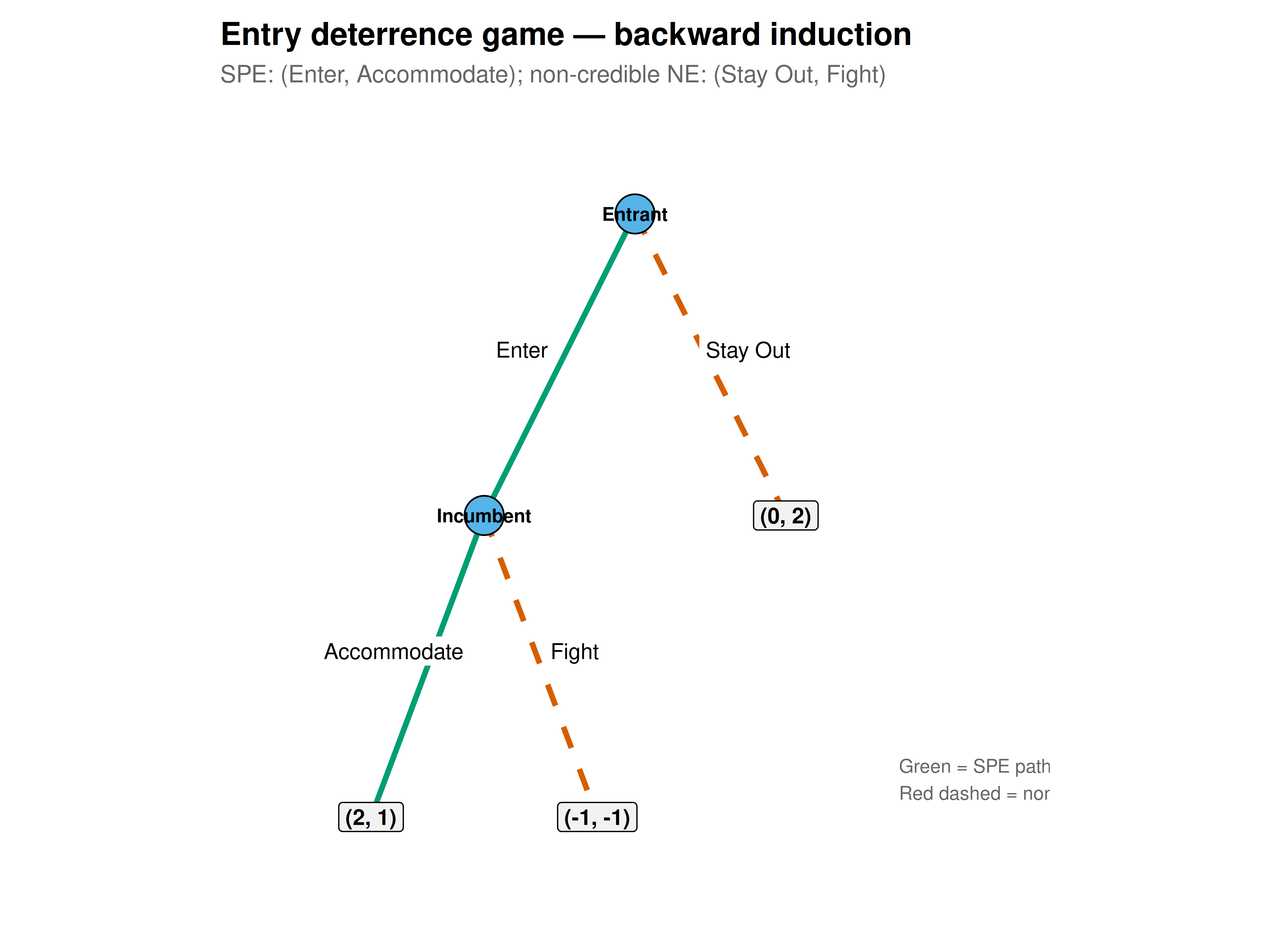
**Entry deterrence game**: Entrant chooses Enter ($E$) or Stay Out ($O$). If Enter, Incumbent chooses Fight ($F$) or Accommodate ($A$).
$$
\text{Payoffs: } (E, A) = (2, 1), \quad (E, F) = (-1, -1), \quad (O) = (0, 2)
$$
The NE "Incumbent fights if entered" is a valid Nash strategy that deters entry, but it fails SPE: if actually faced with entry, fighting yields $-1 < 1$ for the incumbent, so the threat to fight is non-credible.
## R implementation
```{r}
#| label: game-tree-engine
# Represent game tree as a nested list structure
# Each node: list(player, actions, children, payoffs)

# Entry deterrence game
entry_game <- list(
  player = "Entrant",
  actions = c("Enter", "Stay Out"),
  children = list(
    Enter = list(
      player = "Incumbent",
      actions = c("Accommodate", "Fight"),
      children = list(
        Accommodate = list(payoffs = c(Entrant = 2, Incumbent = 1)),
        Fight = list(payoffs = c(Entrant = -1, Incumbent = -1))
      )
    ),
    `Stay Out` = list(payoffs = c(Entrant = 0, Incumbent = 2))
  )
)

# Backward induction solver
backward_induction <- function(node, depth = 0, path = character(0)) {
  indent <- paste(rep("  ", depth), collapse = "")

  # Terminal node

  if (!is.null(node$payoffs)) {
    return(list(payoffs = node$payoffs, path = path))
  }

  # Recursive: solve all children, then pick best for current player
  results <- lapply(names(node$children), function(action) {
    backward_induction(node$children[[action]], depth + 1,
                        c(path, paste0(node$player, ": ", action)))
  })

  # Current player maximises their own payoff
  player <- node$player
  child_payoffs <- sapply(results, function(r) r$payoffs[player])
  best_idx <- which.max(child_payoffs)

  cat(sprintf("%s%s chooses '%s' (payoff %.0f vs alternatives: %s)\n",
              indent, player, names(node$children)[best_idx],
              child_payoffs[best_idx],
              paste(round(child_payoffs[-best_idx], 1), collapse = ", ")))

  results[[best_idx]]
}

cat("=== Entry Deterrence Game — Backward Induction ===\n")
spe <- backward_induction(entry_game)
cat(sprintf("\nSPE outcome: %s\n", paste(spe$path, collapse = " → ")))
cat(sprintf("SPE payoffs: Entrant = %.0f, Incumbent = %.0f\n",
            spe$payoffs["Entrant"], spe$payoffs["Incumbent"]))
```
```{r}
#| label: centipede-game
# Centipede game: alternating players, each can Stop or Continue
# Payoffs grow but the stopper gets a bonus
build_centipede <- function(n_rounds = 6) {
  # Build from the end
  build_node <- function(round, pot_continue, pot_stop) {
    player <- ifelse(round %% 2 == 1, "Player 1", "Player 2")

    if (round > n_rounds) {
      # Terminal: split pot equally
      return(list(payoffs = c(`Player 1` = pot_continue/2, `Player 2` = pot_continue/2)))
    }

    # Stop payoffs: current player gets more
    stop_payoffs <- if (player == "Player 1") {
      c(`Player 1` = pot_stop, `Player 2` = pot_stop - 1)
    } else {
      c(`Player 1` = pot_stop - 1, `Player 2` = pot_stop)
    }

    list(
      player = player,
      actions = c("Stop", "Continue"),
      children = list(
        Stop = list(payoffs = stop_payoffs),
        Continue = build_node(round + 1, pot_continue + 2, pot_stop + 1)
      )
    )
  }

  build_node(1, 2, 1)
}

centipede <- build_centipede(6)
cat("\n=== Centipede Game (6 rounds) — Backward Induction ===\n")
spe_cent <- backward_induction(centipede)
cat(sprintf("\nSPE: %s\n", paste(spe_cent$path, collapse = " → ")))
cat(sprintf("SPE payoffs: P1 = %.0f, P2 = %.0f\n",
            spe_cent$payoffs["Player 1"], spe_cent$payoffs["Player 2"]))
cat("(Backward induction predicts immediate stopping despite mutual gains from continuing)\n")
```
## Static publication-ready figure
```{r}
#| label: fig-game-tree
#| fig-cap: "Figure 1. Entry deterrence game tree with backward induction solution. Green path: subgame-perfect equilibrium (Enter → Accommodate). Red dashed: non-credible threat (Fight). The incumbent's threat to fight deters entry in one Nash equilibrium, but backward induction reveals this threat is not credible — if faced with entry, the rational incumbent accommodates. Okabe-Ito palette."
#| dev: [png, pdf]
#| fig-width: 8
#| fig-height: 6
#| dpi: 300
# Manual layout for the entry deterrence game tree
nodes <- tibble(
  id = c("root", "inc", "stay_out", "accommodate", "fight"),
  label = c("Entrant", "Incumbent", "(0, 2)", "(2, 1)", "(-1, -1)"),
  x = c(0.5, 0.3, 0.7, 0.15, 0.45),
  y = c(0.9, 0.5, 0.5, 0.1, 0.1),
  type = c("decision", "decision", "terminal", "terminal", "terminal")
)

edges <- tibble(
  from_x = c(0.5, 0.5, 0.3, 0.3),
  from_y = c(0.9, 0.9, 0.5, 0.5),
  to_x = c(0.3, 0.7, 0.15, 0.45),
  to_y = c(0.5, 0.5, 0.1, 0.1),
  label = c("Enter", "Stay Out", "Accommodate", "Fight"),
  spe = c(TRUE, FALSE, TRUE, FALSE),
  label_x = c(0.35, 0.65, 0.18, 0.42),
  label_y = c(0.72, 0.72, 0.32, 0.32)
)

p_tree <- ggplot() +
  # Edges
  geom_segment(data = edges, aes(x = from_x, y = from_y, xend = to_x, yend = to_y,
                                   color = spe, linetype = spe),
               linewidth = 1.2, arrow = arrow(length = unit(0.15, "cm"))) +
  # Edge labels
  geom_label(data = edges, aes(x = label_x, y = label_y, label = label),
             size = 3.5, fill = "white", label.size = 0) +
  # Decision nodes
  geom_point(data = filter(nodes, type == "decision"),
             aes(x = x, y = y), size = 8, shape = 21,
             fill = okabe_ito[2], color = "black") +
  geom_text(data = filter(nodes, type == "decision"),
            aes(x = x, y = y, label = label), size = 3, fontface = "bold") +
  # Terminal nodes
  geom_label(data = filter(nodes, type == "terminal"),
             aes(x = x, y = y, label = label), size = 3.5,
             fill = "grey95", fontface = "bold") +
  # SPE path annotation
  annotate("text", x = 0.85, y = 0.15,
           label = "Green = SPE path\nRed dashed = non-credible",
           size = 3, color = "grey40", hjust = 0) +
  scale_color_manual(values = c("TRUE" = okabe_ito[3], "FALSE" = okabe_ito[6]),
                      guide = "none") +
  scale_linetype_manual(values = c("TRUE" = "solid", "FALSE" = "dashed"),
                         guide = "none") +
  coord_fixed(xlim = c(0, 1), ylim = c(0, 1)) +
  labs(
    title = "Entry deterrence game — backward induction",
    subtitle = "SPE: (Enter, Accommodate); non-credible NE: (Stay Out, Fight)"
  ) +
  theme_publication() +
  theme(axis.text = element_blank(), axis.title = element_blank(),
        axis.ticks = element_blank(), axis.line = element_blank(),
        panel.grid = element_blank())

p_tree
```
## Interactive figure
```{r}
#| label: fig-centipede-payoffs
# Visualize centipede game payoffs at each stopping point
n_rounds <- 10
stop_payoffs <- tibble(
  round = 1:n_rounds,
  stopper = ifelse(1:n_rounds %% 2 == 1, "Player 1", "Player 2"),
  stopper_payoff = 1:n_rounds,
  other_payoff = 0:(n_rounds - 1),
  continue_both = (1:n_rounds + 1)  # payoff if game continues to end
) |>
  mutate(text = paste0("Round ", round, "\nStopper: ", stopper,
                       "\nStopper gets: ", stopper_payoff,
                       "\nOther gets: ", other_payoff))

p_cent <- ggplot(stop_payoffs) +
  geom_line(aes(x = round, y = stopper_payoff, color = "Stopper"),
            linewidth = 1) +
  geom_line(aes(x = round, y = other_payoff, color = "Other player"),
            linewidth = 1) +
  geom_line(aes(x = round, y = continue_both, color = "Mutual continuation"),
            linewidth = 1, linetype = "dashed") +
  geom_point(aes(x = round, y = stopper_payoff, text = text), color = okabe_ito[6], size = 3) +
  scale_color_manual(values = c("Stopper" = okabe_ito[6], "Other player" = okabe_ito[5],
                                  "Mutual continuation" = okabe_ito[3]),
                      name = "Payoff to") +
  labs(
    title = "Centipede game — payoffs at each stopping point",
    subtitle = "Backward induction predicts stopping at round 1 despite mutual gains from continuing",
    x = "Round (stopping point)", y = "Payoff"
  ) +
  theme_publication()

ggplotly(p_cent, tooltip = "text") |>
  config(displaylogo = FALSE,
         modeBarButtonsToRemove = c("select2d", "lasso2d"))
```
## Interpretation
The entry deterrence game illustrates the core insight of subgame-perfect equilibrium: not all Nash equilibria are equally plausible. The strategy profile (Stay Out, Fight if Enter) is a Nash equilibrium — given that the incumbent will fight, staying out is the entrant's best response, and given that the entrant stays out, the incumbent's threat to fight is never tested. But backward induction reveals this equilibrium relies on a non-credible threat: if actually faced with entry, the rational incumbent prefers to accommodate (payoff 1) over fight (payoff $-1$). SPE eliminates this implausible equilibrium, predicting (Enter, Accommodate) as the unique credible outcome. The centipede game pushes this logic to its limit: backward induction predicts that Player 1 stops immediately at round 1, forgoing the much larger payoffs available through mutual cooperation. This prediction is notoriously at odds with experimental evidence — real players frequently continue for several rounds, suggesting that backward induction, while logically impeccable, may require unrealistic levels of strategic sophistication or common knowledge of rationality. This tension between the theoretical elegance of SPE and the messiness of actual behaviour motivates much of behavioural game theory, including models of bounded rationality, $\epsilon$-equilibrium, and quantal response equilibrium.
## Extensions & related tutorials
- [Dominant strategies and iterated elimination](../dominant-strategies-iterated-elimination/) — the normal-form precursor to backward induction.
- [Mixed-strategy Nash equilibrium in 2×2 games](../nash-equilibrium-mixed/) — when pure-strategy analysis is insufficient.
- [The ultimatum game — bargaining and fairness](../../classical-games/ultimatum-game/) — SPE vs experimental evidence.
- [Signaling games and perfect Bayesian equilibrium](../signaling-games-pbe/) — extending SPE to games with incomplete information.
- [Cuban Missile Crisis as a signaling game](../../real-world-data-applications/cuban-missile-crisis-signaling-game/) — applied sequential reasoning.
## References
::: {#refs}
:::