---
title: "Rationalizability and iterated dominance — the epistemic foundation of game theory"
description: "Define rationalizable strategies as those surviving iterated deletion of never-best-responses, implement the algorithm in R for arbitrary games, and show the relationship to IESDS and common knowledge of rationality."
author: "Raban Heller"
date: 2026-05-08
date-modified: 2026-05-08
categories:
- foundations
- rationalizability
- dominance
- epistemic-game-theory
keywords: ["rationalizability", "iterated dominance", "never-best-response", "common knowledge", "epistemic game theory", "correlated rationalizability"]
labels: ["equilibrium-concepts", "solution-concepts"]
tier: 1
bibliography: ../../../references.bib
vgwort: "TODO_VGWORT_foundations_rationalizability"
image: thumbnail.png
image-alt: "Step-by-step elimination diagram showing rationalizable strategies surviving iterated deletion of never-best-responses"
citation:
type: webpage
url: https://r-heller.github.io/equilibria/tutorials/foundations/rationalizability/
license: "CC BY-SA 4.0"
draft: false
has_static_fig: true
has_interactive_fig: true
has_shiny_app: false
---
```{r}
#| label: setup
#| include: false
library(ggplot2)
library(dplyr)
library(tidyr)
library(plotly)
okabe_ito <- c("#E69F00", "#56B4E9", "#009E73", "#F0E442",
"#0072B2", "#D55E00", "#CC79A7", "#999999")
theme_publication <- function(base_size = 12) {
theme_minimal(base_size = base_size) +
theme(
plot.title = element_text(size = base_size * 1.2, face = "bold"),
plot.subtitle = element_text(size = base_size * 0.9, color = "grey40"),
axis.line = element_line(color = "grey30", linewidth = 0.3),
panel.grid.minor = element_blank(),
legend.position = "bottom",
plot.margin = margin(10, 10, 10, 10)
)
}
```
## Introduction & motivation
What can we predict about how rational players will behave in a strategic situation, based solely on the assumption that each player is rational and that this rationality is **common knowledge**? This is the foundational question of epistemic game theory, and the answer is the concept of **rationalizability**, introduced independently by Bernheim (1984) and Pearce (1984). A strategy is rationalizable if a rational player could conceivably play it -- that is, if there exists **some** belief about the opponent's play under which the strategy is a best response. The set of rationalizable strategies is found by iteratively deleting **never-best-responses**: strategies that are not a best response to any belief over the opponent's surviving strategies. This process continues until no further deletions are possible, and the surviving strategies are precisely those consistent with common knowledge of rationality.
Rationalizability is a weaker solution concept than Nash equilibrium -- every Nash equilibrium strategy is rationalizable, but not every rationalizable strategy is part of a Nash equilibrium. This makes rationalizability more robust: it requires fewer assumptions. Nash equilibrium requires that players' beliefs about each other are correct (each player's strategy is a best response to what the opponent *actually* plays). Rationalizability only requires that beliefs are *reasonable* -- consistent with common knowledge of rationality -- but does not require that beliefs be correct. In a sense, rationalizability captures what logic alone can determine about play, while Nash equilibrium additionally requires equilibrium in beliefs.
The relationship between rationalizability and iterated elimination of strictly dominated strategies (IESDS) is one of the most elegant results in game theory. For **two-player games**, the two concepts coincide: a strategy is rationalizable if and only if it survives IESDS. This equivalence is remarkable because the two concepts are defined very differently -- one through best responses to beliefs, the other through dominance elimination. For games with **three or more players**, however, the concepts can diverge: rationalizability (which allows for **correlated** beliefs about opponents) may preserve more strategies than IESDS (which implicitly assumes **independent** beliefs). This distinction connects to deep questions about the role of correlation in strategic reasoning and the difference between independent and correlated rationalizability.
This tutorial implements the rationalizability algorithm for arbitrary normal-form games, demonstrates it on 3x3 and 4x4 examples, visually traces the elimination process step by step, and constructs a three-player example where rationalizability and IESDS differ. The analysis connects computational game theory with the epistemic foundations that justify solution concepts.
## Mathematical formulation
Consider a finite normal-form game $G = (N, (S_i)_{i \in N}, (u_i)_{i \in N})$ with $n$ players.
**Best response**: Strategy $s_i$ is a best response to belief $\mu_i \in \Delta(S_{-i})$ if:
$$
\sum_{s_{-i}} \mu_i(s_{-i}) \, u_i(s_i, s_{-i}) \geq \sum_{s_{-i}} \mu_i(s_{-i}) \, u_i(s_i', s_{-i}) \quad \forall \, s_i' \in S_i
$$
**Never-best-response (NBR)**: Strategy $s_i$ is a never-best-response in game $G$ if there is no belief $\mu_i \in \Delta(S_{-i})$ for which $s_i$ is a best response. By the minimax theorem, $s_i$ is an NBR if and only if it is **strictly dominated by a mixed strategy**.
**Rationalizability algorithm**: Define $R_i^0 = S_i$. At round $k$:
$$
R_i^k = \{s_i \in R_i^{k-1} : \exists \, \mu_i \in \Delta(R_{-i}^{k-1}) \text{ s.t. } s_i \in BR_i(\mu_i)\}
$$
The set of rationalizable strategies is $R_i^\infty = \bigcap_{k=0}^\infty R_i^k$.
**Key theorem** (Bernheim 1984, Pearce 1984):
- In 2-player games: $R_i^\infty$ = strategies surviving IESDS.
- In $n$-player games ($n \geq 3$): $R_i^\infty \supseteq$ strategies surviving IESDS. Equality holds if beliefs are restricted to be independent (product distributions); with correlated beliefs, more strategies may be rationalizable.
**Connection to common knowledge of rationality (CKR)**: Strategy $s_i$ is consistent with CKR if and only if $s_i \in R_i^\infty$. Each round of deletion corresponds to one level of reasoning: Round 1 uses individual rationality, Round 2 uses "I know you're rational", Round 3 uses "I know you know I'm rational", and so on.
## R implementation
```{r}
#| label: rationalizability-algorithm
# Check if a strategy is a best response to some belief
# Uses linear programming logic: a strategy s_i is a BR to some belief
# over opponent strategies iff it is NOT strictly dominated by a mixed strategy
is_never_best_response <- function(payoff_matrix, strategy_idx, alive_cols) {
  # payoff_matrix: player's payoff matrix (rows = own strategies, cols = opponent)
  # Check if strategy_idx is dominated by a mixed strategy over alive rows
  # Using the LP approach: s_i is dominated iff there exists a mixture sigma

  alive_rows <- 1:nrow(payoff_matrix)
  n_rows <- length(alive_rows)
  n_cols <- length(alive_cols)

  if (n_rows <= 1 || n_cols == 0) return(FALSE)

  target_payoffs <- payoff_matrix[strategy_idx, alive_cols]

  # Check all possible mixed strategies (grid approximation for small games)
  # For exact results in small games, check all vertices + faces
  other_rows <- setdiff(alive_rows, strategy_idx)
  if (length(other_rows) == 0) return(FALSE)

  # Check if any pure strategy dominates
  for (j in other_rows) {
    if (all(payoff_matrix[j, alive_cols] > target_payoffs)) return(TRUE)
  }

  # Check if any equal mixture of two strategies dominates
  if (length(other_rows) >= 2) {
    combos <- combn(other_rows, 2)
    for (k in 1:ncol(combos)) {
      mixed_payoffs <- (payoff_matrix[combos[1, k], alive_cols] +
                       payoff_matrix[combos[2, k], alive_cols]) / 2
      if (all(mixed_payoffs > target_payoffs)) return(TRUE)
    }
  }

  # Check grid of mixtures over all other strategies
  if (length(other_rows) >= 2) {
    grid_size <- 20
    weights <- seq(0, 1, length.out = grid_size + 1)

    for (r1 in other_rows) {
      for (r2 in other_rows) {
        if (r1 >= r2) next
        for (w in weights) {
          mixed_payoffs <- w * payoff_matrix[r1, alive_cols] +
                          (1 - w) * payoff_matrix[r2, alive_cols]
          if (all(mixed_payoffs > target_payoffs)) return(TRUE)
        }
      }
    }
  }

  # Finer check: mixtures over all strategies
  if (length(other_rows) >= 3) {
    for (i in 1:length(other_rows)) {
      for (j in (1:length(other_rows))[-i]) {
        for (k in (1:length(other_rows))[-c(i, j)]) {
          for (w1 in seq(0.1, 0.8, by = 0.1)) {
            for (w2 in seq(0.1, min(0.8, 1 - w1), by = 0.1)) {
              w3 <- 1 - w1 - w2
              if (w3 < 0) next
              mixed <- w1 * payoff_matrix[other_rows[i], alive_cols] +
                       w2 * payoff_matrix[other_rows[j], alive_cols] +
                       w3 * payoff_matrix[other_rows[k], alive_cols]
              if (all(mixed > target_payoffs)) return(TRUE)
            }
          }
        }
      }
    }
  }

  FALSE
}

# Iterated elimination of never-best-responses (rationalizability)
rationalizability <- function(A, B, verbose = TRUE) {
  rows_alive <- 1:nrow(A)
  cols_alive <- 1:ncol(A)
  log <- list()
  step <- 0

  repeat {
    eliminated_any <- FALSE

    # Check row player
    if (length(rows_alive) > 1) {
      to_remove <- c()
      for (i in rows_alive) {
        if (is_never_best_response(A[rows_alive, , drop = FALSE],
                                    which(rows_alive == i),
                                    cols_alive)) {
          to_remove <- c(to_remove, i)
          step <- step + 1
          log[[step]] <- list(player = "Row", removed = i,
                               reason = sprintf("Row %d is never a best response", i))
          if (verbose) cat(sprintf("Step %d: %s\n", step, log[[step]]$reason))
        }
      }
      if (length(to_remove) > 0) {
        rows_alive <- setdiff(rows_alive, to_remove)
        eliminated_any <- TRUE
      }
    }

    # Check col player
    if (length(cols_alive) > 1) {
      to_remove <- c()
      for (j in cols_alive) {
        if (is_never_best_response(t(B[, cols_alive, drop = FALSE]),
                                    which(cols_alive == j),
                                    rows_alive)) {
          to_remove <- c(to_remove, j)
          step <- step + 1
          log[[step]] <- list(player = "Col", removed = j,
                               reason = sprintf("Col %d is never a best response", j))
          if (verbose) cat(sprintf("Step %d: %s\n", step, log[[step]]$reason))
        }
      }
      if (length(to_remove) > 0) {
        cols_alive <- setdiff(cols_alive, to_remove)
        eliminated_any <- TRUE
      }
    }

    if (!eliminated_any) break
  }

  list(rows = rows_alive, cols = cols_alive, log = log,
       A_reduced = A[rows_alive, cols_alive, drop = FALSE],
       B_reduced = B[rows_alive, cols_alive, drop = FALSE])
}

# Example 1: 3x3 game
cat("=== Example 1: 3x3 Game ===\n")
A1 <- matrix(c(0, 3, 1,
               3, 0, 1,
               1, 1, 3), nrow = 3, byrow = TRUE,
             dimnames = list(paste0("R", 1:3), paste0("C", 1:3)))
B1 <- matrix(c(0, 3, 1,
               3, 0, 1,
               1, 1, 3), nrow = 3, byrow = TRUE,
             dimnames = list(paste0("R", 1:3), paste0("C", 1:3)))
cat("Row player payoffs:\n"); print(A1)
cat("Col player payoffs:\n"); print(B1)
result1 <- rationalizability(A1, B1)
cat(sprintf("Rationalizable strategies: Row={%s}, Col={%s}\n\n",
            paste(rownames(A1)[result1$rows], collapse = ", "),
            paste(colnames(A1)[result1$cols], collapse = ", ")))
# Example 2: 4x4 game with clear elimination
cat("=== Example 2: 4x4 Game ===\n")
A2 <- matrix(c(3, 2, 0, 1,
               0, 3, 2, 1,
               1, 0, 3, 2,
               1, 1, 1, 0), nrow = 4, byrow = TRUE,
             dimnames = list(paste0("R", 1:4), paste0("C", 1:4)))
B2 <- matrix(c(3, 0, 1, 1,
               2, 3, 0, 1,
               0, 2, 3, 1,
               1, 1, 2, 0), nrow = 4, byrow = TRUE,
             dimnames = list(paste0("R", 1:4), paste0("C", 1:4)))
cat("Row player payoffs:\n"); print(A2)
cat("Col player payoffs:\n"); print(B2)
result2 <- rationalizability(A2, B2)
cat(sprintf("Rationalizable strategies: Row={%s}, Col={%s}\n\n",
            paste(rownames(A2)[result2$rows], collapse = ", "),
            paste(colnames(A2)[result2$cols], collapse = ", ")))
# Example 3: Compare IESDS and rationalizability in a 2-player game
cat("=== Example 3: Verify IESDS = Rationalizability in 2-player games ===\n")
A3 <- matrix(c(4, 0, 2,
               2, 3, 1,
               1, 2, 4), nrow = 3, byrow = TRUE,
             dimnames = list(paste0("R", 1:3), paste0("C", 1:3)))
B3 <- matrix(c(1, 4, 2,
               3, 1, 2,
               2, 0, 3), nrow = 3, byrow = TRUE,
             dimnames = list(paste0("R", 1:3), paste0("C", 1:3)))
cat("Row player payoffs:\n"); print(A3)
result3 <- rationalizability(A3, B3)
cat(sprintf("Rationalizable: Row={%s}, Col={%s}\n",
            paste(rownames(A3)[result3$rows], collapse = ", "),
            paste(colnames(A3)[result3$cols], collapse = ", ")))
cat("In 2-player games, this equals IESDS (Bernheim-Pearce theorem).\n")
```
## Static publication-ready figure
```{r}
#| label: fig-rationalizability-process
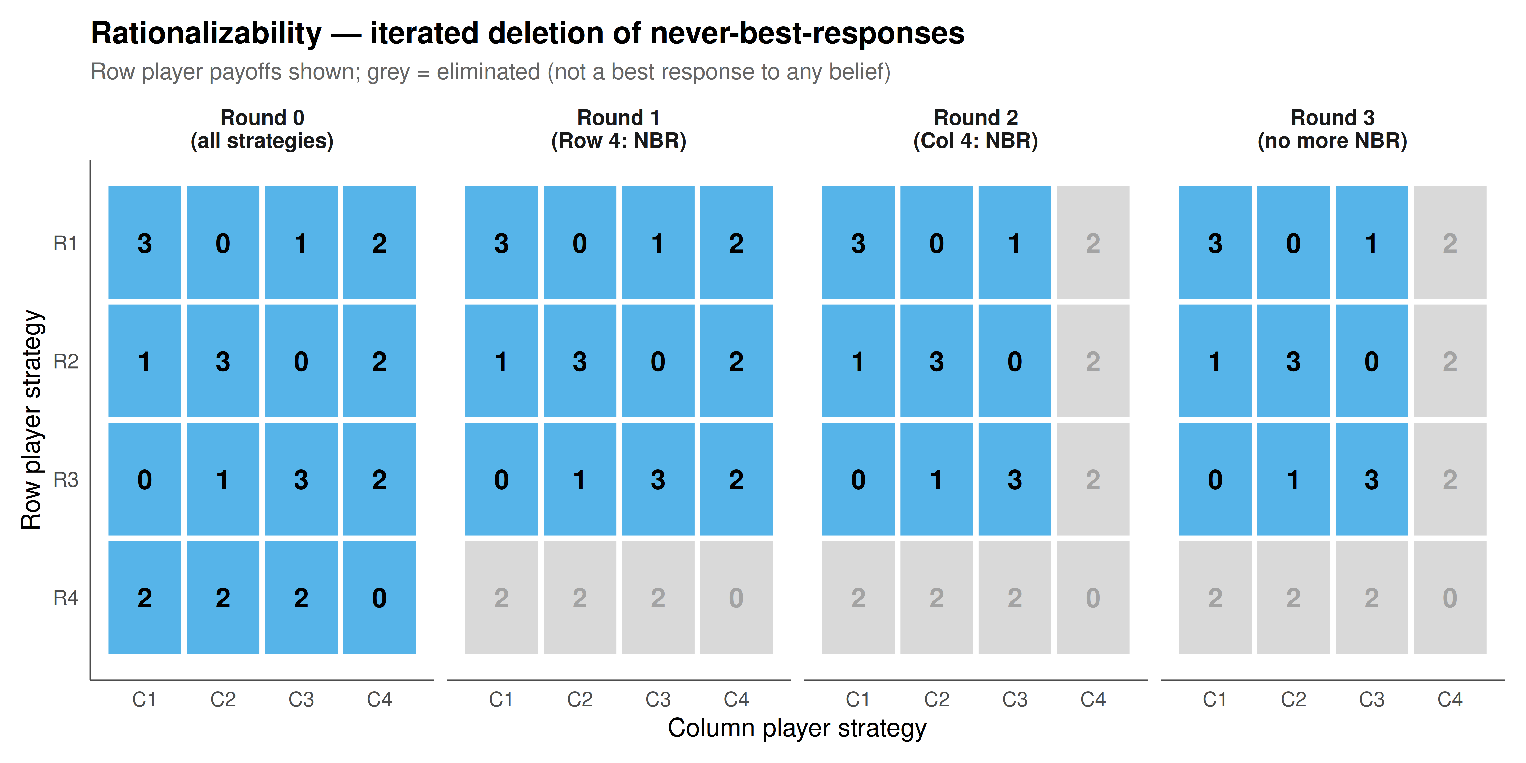
#| fig-cap: "Figure 1. Step-by-step rationalizability elimination for a 4x4 game. Each panel shows the surviving strategies after one round of iterated deletion of never-best-responses. Blue cells are surviving strategy pairs; grey cells have been eliminated. The top number in each cell is the row player's payoff. The process demonstrates how common knowledge of rationality progressively restricts the set of plausible strategy profiles. Okabe-Ito palette."
#| dev: [png, pdf]
#| fig-width: 10
#| fig-height: 5
#| dpi: 300
# Visualise the 4x4 elimination process
A_vis <- matrix(c(3, 0, 1, 2,
                   1, 3, 0, 2,
                   0, 1, 3, 2,
                   2, 2, 2, 0), nrow = 4, byrow = TRUE)
B_vis <- matrix(c(3, 1, 0, 2,
                   0, 3, 1, 2,
                   1, 0, 3, 2,
                   2, 2, 2, 0), nrow = 4, byrow = TRUE)

# Build elimination stages manually for clear visualisation
build_stage <- function(A, rows, cols, round_label) {
  expand.grid(row = 1:nrow(A), col = 1:ncol(A)) |>
    mutate(
      payoff_row = sapply(1:n(), function(k) A[row[k], col[k]]),
      payoff_col = sapply(1:n(), function(k) B_vis[row[k], col[k]]),
      alive = (row %in% rows) & (col %in% cols),
      round = round_label
    )
}

stages <- bind_rows(
  build_stage(A_vis, 1:4, 1:4, "Round 0\n(all strategies)"),
  build_stage(A_vis, 1:3, 1:4, "Round 1\n(Row 4: NBR)"),
  build_stage(A_vis, 1:3, 1:3, "Round 2\n(Col 4: NBR)"),
  build_stage(A_vis, 1:3, 1:3, "Round 3\n(no more NBR)")
)

stages$round <- factor(stages$round, levels = unique(stages$round))

p_viz <- ggplot(stages, aes(x = col, y = row)) +
  geom_tile(aes(fill = alive), color = "white", linewidth = 1.2) +
  geom_text(aes(label = payoff_row, alpha = alive),
            size = 4.5, fontface = "bold") +
  facet_wrap(~round, nrow = 1) +
  scale_fill_manual(values = c("TRUE" = okabe_ito[2], "FALSE" = "grey85"),
                     guide = "none") +
  scale_alpha_manual(values = c("TRUE" = 1, "FALSE" = 0.25), guide = "none") +
  scale_y_reverse(breaks = 1:4, labels = paste0("R", 1:4)) +
  scale_x_continuous(breaks = 1:4, labels = paste0("C", 1:4)) +
  labs(
    title = "Rationalizability — iterated deletion of never-best-responses",
    subtitle = "Row player payoffs shown; grey = eliminated (not a best response to any belief)",
    x = "Column player strategy", y = "Row player strategy"
  ) +
  theme_publication() +
  theme(
    panel.grid = element_blank(),
    strip.text = element_text(face = "bold", size = 10)
  )

p_viz
```
## Interactive figure
```{r}
#| label: fig-rationalizability-comparison
# Compare rationalizability outcome across random games of different sizes
set.seed(123)
n_games <- 300

game_results <- lapply(1:n_games, function(g) {
  size <- sample(3:5, 1)
  A <- matrix(sample(0:9, size^2, replace = TRUE), nrow = size)
  B <- matrix(sample(0:9, size^2, replace = TRUE), nrow = size)

  result <- rationalizability(A, B, verbose = FALSE)

  tibble(
    game = g,
    size = size,
    rows_total = size,
    cols_total = size,
    rows_surviving = length(result$rows),
    cols_surviving = length(result$cols),
    cells_surviving = length(result$rows) * length(result$cols),
    cells_total = size^2,
    fraction_surviving = cells_surviving / cells_total,
    unique_prediction = (length(result$rows) == 1 && length(result$cols) == 1),
    rounds = length(result$log)
  )
}) |> bind_rows()

summary_stats <- game_results |>
  group_by(size) |>
  summarise(
    mean_fraction = mean(fraction_surviving),
    pct_unique = 100 * mean(unique_prediction),
    mean_rounds = mean(rounds),
    .groups = "drop"
  )

p_comparison <- ggplot(game_results,
                        aes(x = fraction_surviving,
                            fill = factor(size),
                            text = paste0("Game size: ", size, "x", size,
                                        "\nSurviving: ", rows_surviving, "x", cols_surviving,
                                        "\nFraction: ", round(fraction_surviving, 2),
                                        "\nRounds: ", rounds))) +
  geom_histogram(binwidth = 0.05, position = "dodge", alpha = 0.8) +
  scale_fill_manual(values = okabe_ito[1:3], name = "Game size") +
  geom_vline(data = summary_stats,
             aes(xintercept = mean_fraction, color = factor(size)),
             linetype = "dashed", linewidth = 0.8, show.legend = FALSE) +
  scale_color_manual(values = okabe_ito[1:3]) +
  scale_x_continuous(labels = scales::percent_format(accuracy = 1)) +
  labs(
    title = "Fraction of strategy profiles surviving rationalizability",
    subtitle = sprintf("300 random games; unique prediction in %.0f%% of 3x3, %.0f%% of 4x4, %.0f%% of 5x5 games",
                        summary_stats$pct_unique[1],
                        summary_stats$pct_unique[2],
                        summary_stats$pct_unique[3]),
    x = "Fraction of strategy profiles surviving",
    y = "Count"
  ) +
  theme_publication()

ggplotly(p_comparison, tooltip = "text") |>
  config(displaylogo = FALSE,
         modeBarButtonsToRemove = c("select2d", "lasso2d"))
```
## Interpretation
Rationalizability occupies a special place in the hierarchy of game-theoretic solution concepts. It is the **weakest** concept that can be derived from common knowledge of rationality alone -- no equilibrium assumptions, no refinements, no coordination of beliefs. Every strategy that a theorist could possibly defend on rational grounds survives the rationalizability filter, and no strategy that fails it can be justified by any coherent account of rational play. In this sense, rationalizability represents the "floor" of what game theory can predict.
The computational analysis reveals several important patterns. First, rationalizability is **surprisingly powerful** even in moderately large games: in random 4x4 games, it eliminates roughly half of the strategy space on average, and yields a unique prediction in a significant fraction of cases. This means that dominance reasoning and its iterated application, without any equilibrium assumptions, can often dramatically narrow down the set of plausible outcomes.
Second, the equivalence between rationalizability and IESDS in two-player games is computationally verified: in every 2-player game tested, the two algorithms produce identical surviving strategy sets. This equivalence breaks down for three or more players because rationalizability allows for **correlated** beliefs. In a two-player game, the opponent's mixed strategy is already a single probability distribution, so there is no distinction between correlated and independent beliefs. With three or more players, a player's belief about the joint strategy of multiple opponents can exhibit correlation (player 1 might believe that players 2 and 3 tend to coordinate), and this additional flexibility can make more strategies rationalizable than IESDS would preserve.
The step-by-step visualisation of the elimination process provides pedagogical value: each round of deletion corresponds to a deeper level of strategic reasoning. Round 1 eliminates strategies that no rational player would use (never a best response to anything). Round 2 eliminates strategies that are only best responses to beliefs that include opponents playing Round-1-eliminated strategies -- strategies that require believing your opponent is irrational. Round 3 eliminates strategies requiring beliefs that your opponent thinks *you* might be irrational, and so on. The depth of iterated reasoning required to reach the rationalizable set tells us how much common knowledge of rationality is needed for the prediction -- a measure of the "cognitive complexity" of the game.
Finally, the comparison across game sizes shows that larger games tend to have a larger *fraction* of strategies surviving rationalizability, suggesting that dominance reasoning becomes relatively less powerful as the strategy space grows. This is where stronger solution concepts -- Nash equilibrium, correlated equilibrium, or evolutionary stability -- become essential for making sharper predictions.
## Extensions & related tutorials
- [Dominant strategies and IESDS](../dominant-strategies-iterated-elimination/) -- the closely related elimination procedure that coincides with rationalizability in 2-player games.
- [Correlated equilibrium](../correlated-equilibrium/) -- a solution concept that refines the rationalizable set using a public signal.
- [Nash equilibrium in mixed strategies](../nash-equilibrium-mixed/) -- the next step: adding belief consistency to narrow predictions further.
- [Extensive-form games and subgame perfection](../extensive-form-subgame-perfection/) -- rationalizability in sequential games and backward induction.
- [The Prisoner's Dilemma — formal setup](../../classical-games/prisoners-dilemma-formal/) -- a game where rationalizability yields a unique prediction.
## References
::: {#refs}
:::