---
title: "From von Neumann to Nash — a mathematical timeline of game theory"
description: "Interactive timeline of key results from the 1928 minimax theorem through Nash's 1950-51 equilibrium existence proof, with R visualizations of each milestone's mathematical contribution to game theory."
author: "Raban Heller"
date: 2026-05-08
date-modified: 2026-05-08
categories:
- history-of-gt-mathematics
- timeline
- mathematical-history
keywords: ["game theory history", "von Neumann", "Nash equilibrium", "minimax theorem", "Zermelo", "Borel", "mathematical timeline", "R"]
labels: ["history", "foundations"]
tier: 1
bibliography: ../../../references.bib
vgwort: "TODO_VGWORT_history-of-gt-mathematics_von-neumann-to-nash-timeline"
image: thumbnail.png
image-alt: "Interactive timeline of game theory milestones from 1913 to 1953 with mathematical contributions"
citation:
type: webpage
url: https://r-heller.github.io/equilibria/tutorials/history-of-gt-mathematics/von-neumann-to-nash-timeline/
license: "CC BY-SA 4.0"
draft: false
has_static_fig: true
has_interactive_fig: true
has_shiny_app: false
---
```{r}
#| label: setup
#| include: false
library(ggplot2)
library(dplyr)
library(tidyr)
library(plotly)
okabe_ito <- c("#E69F00", "#56B4E9", "#009E73", "#F0E442",
"#0072B2", "#D55E00", "#CC79A7", "#999999")
theme_publication <- function(base_size = 12) {
theme_minimal(base_size = base_size) +
theme(
plot.title = element_text(size = base_size * 1.2, face = "bold"),
plot.subtitle = element_text(size = base_size * 0.9, color = "grey40"),
axis.line = element_line(color = "grey30", linewidth = 0.3),
panel.grid.minor = element_blank(),
legend.position = "bottom",
plot.margin = margin(10, 10, 10, 10)
)
}
```
## Introduction & motivation
Game theory did not emerge fully formed from a single mind. Its mathematical foundations were laid across four decades by a remarkable sequence of thinkers — from Ernst Zermelo's 1913 theorem on chess to John Nash's 1951 proof that every finite game has an equilibrium in mixed strategies. Each milestone built on its predecessors, gradually expanding the scope of strategic analysis from perfect-information parlour games to the general theory of strategic interaction that now pervades economics, political science, biology, and computer science. **Zermelo (1913)** proved that chess is determined: one player has a winning strategy or both can force a draw. **Emile Borel (1921-27)** studied mixed strategies for small games but conjectured that minimax solutions might not always exist. **John von Neumann (1928)** proved the minimax theorem for two-person zero-sum games, overturning Borel's conjecture and establishing the first general existence result in game theory. **Von Neumann and Morgenstern (1944)** published *Theory of Games and Economic Behavior*, introducing expected utility theory, the extensive form, and the characteristic function for cooperative games — transforming game theory from a mathematical curiosity into a framework for social science. **John Nash (1950-51)** made the decisive leap to non-cooperative, non-zero-sum games: his equilibrium concept and existence proof (using Brouwer's or Kakutani's fixed point theorem) showed that every finite game has a strategic equilibrium, inaugurating the modern era of game theory. This tutorial builds an interactive timeline of these milestones and implements the core mathematical idea behind each one in R, demonstrating how the field evolved from specific results about particular games to a universal theory of strategic interaction.
## Mathematical formulation
The key theorems in chronological order:
**Zermelo's theorem (1913)**: In any finite two-player game of perfect information with no chance moves, either player 1 has a winning strategy, player 2 has a winning strategy, or both can force a draw.
**Von Neumann's minimax theorem (1928)**: For any two-person zero-sum game with finite strategy sets $S_1, S_2$ and payoff matrix $A$:
$$
\max_{p \in \Delta(S_1)} \min_{q \in \Delta(S_2)} p^T A q = \min_{q \in \Delta(S_2)} \max_{p \in \Delta(S_1)} p^T A q = v^*
$$
where $\Delta(S)$ is the set of mixed strategies (probability distributions) over $S$.
**Nash's existence theorem (1950)**: Every finite game $\Gamma = (N, (S_i)_{i \in N}, (u_i)_{i \in N})$ possesses at least one Nash equilibrium in mixed strategies. A strategy profile $\sigma^*$ is a NE if for all $i$ and all $\sigma_i$:
$$
u_i(\sigma_i^*, \sigma_{-i}^*) \geq u_i(\sigma_i, \sigma_{-i}^*)
$$
Nash's proof constructs a continuous mapping $f: \prod_i \Delta(S_i) \to \prod_i \Delta(S_i)$ whose fixed points (guaranteed by Kakutani's theorem) are exactly the Nash equilibria.
## R implementation
```{r}
#| label: timeline-data-and-demos
# --- Timeline data ---
milestones <- tibble(
  year = c(1913, 1921, 1928, 1937, 1944, 1950, 1951, 1953),
  author = c("Zermelo", "Borel", "von Neumann", "von Neumann",
             "von Neumann &\nMorgenstern", "Nash", "Nash", "Shapley"),
  title = c(
    "Theorem on chess\n(backward induction)",
    "Mixed strategies for\nsmall games",
    "Minimax theorem\n(zero-sum games)",
    "Expected utility &\nfixed point approach",
    "Theory of Games\nand Economic Behavior",
    "Equilibrium points in\nn-person games (PNAS)",
    "Non-cooperative\ngames (Annals of Math)",
    "A value for\nn-person games"
  ),
  category = c("Perfect information", "Mixed strategies", "Zero-sum",
               "Foundations", "Foundations", "Non-cooperative",
               "Non-cooperative", "Cooperative"),
  importance = c(3, 2, 5, 3, 5, 5, 5, 4)
)

cat("=== Key Milestones in Game Theory (1913-1953) ===\n")
milestones |>
  mutate(title = gsub("\n", " ", title)) |>
  select(year, author, title, category) |>
  print(n = 10)
# --- Demo 1: Minimax theorem (von Neumann 1928) ---
cat("\n=== Von Neumann's Minimax Theorem: Matching Pennies ===\n")
A <- matrix(c(1, -1, -1, 1), nrow = 2, byrow = TRUE)
cat("Payoff matrix A:\n")
print(A)
# Analytical solution: p* = q* = (0.5, 0.5), v* = 0
cat("Minimax value: 0\n")
cat("Optimal strategies: p* = (0.5, 0.5), q* = (0.5, 0.5)\n")
# Verify: maximin = minimax
p_grid <- seq(0, 1, 0.01)
maximin_values <- sapply(p_grid, function(p) {
  pvec <- c(p, 1 - p)
  min(pvec %*% A)
})
minimax_values <- sapply(p_grid, function(q) {
  qvec <- c(q, 1 - q)
  max(A %*% qvec)
})
cat(sprintf("Maximin = %.3f at p = %.2f\n",
            max(maximin_values), p_grid[which.max(maximin_values)]))
cat(sprintf("Minimax = %.3f at q = %.2f\n",
            min(minimax_values), p_grid[which.min(minimax_values)]))
# --- Demo 2: Nash equilibrium (Nash 1950) ---
cat("\n=== Nash Equilibrium: Battle of the Sexes ===\n")
# Player 1 payoffs
A1 <- matrix(c(3, 0, 0, 2), nrow = 2, byrow = TRUE)
# Player 2 payoffs
A2 <- matrix(c(2, 0, 0, 3), nrow = 2, byrow = TRUE)
cat("Player 1 payoffs:\n"); print(A1)
cat("Player 2 payoffs:\n"); print(A2)
# Find mixed NE: p = P(player 1 chooses Opera)
# Player 2 indifferent: 2p + 0(1-p) = 0p + 3(1-p) => 2p = 3 - 3p => p = 3/5
# Player 1 indifferent: 3q + 0(1-q) = 0q + 2(1-q) => 3q = 2 - 2q => q = 2/5
p_ne <- 3/5; q_ne <- 2/5
cat(sprintf("Mixed NE: p(Opera|P1) = %.2f, q(Opera|P2) = %.2f\n", p_ne, q_ne))
eu1 <- p_ne * q_ne * 3 + (1-p_ne) * (1-q_ne) * 2
cat(sprintf("Expected payoff at mixed NE: P1 = %.2f, P2 = %.2f\n", eu1, eu1))
cat("Pure NE: (Opera, Opera) with payoffs (3,2) and (Football, Football) with (2,3)\n")
```
## Static publication-ready figure
```{r}
#| label: fig-gt-timeline
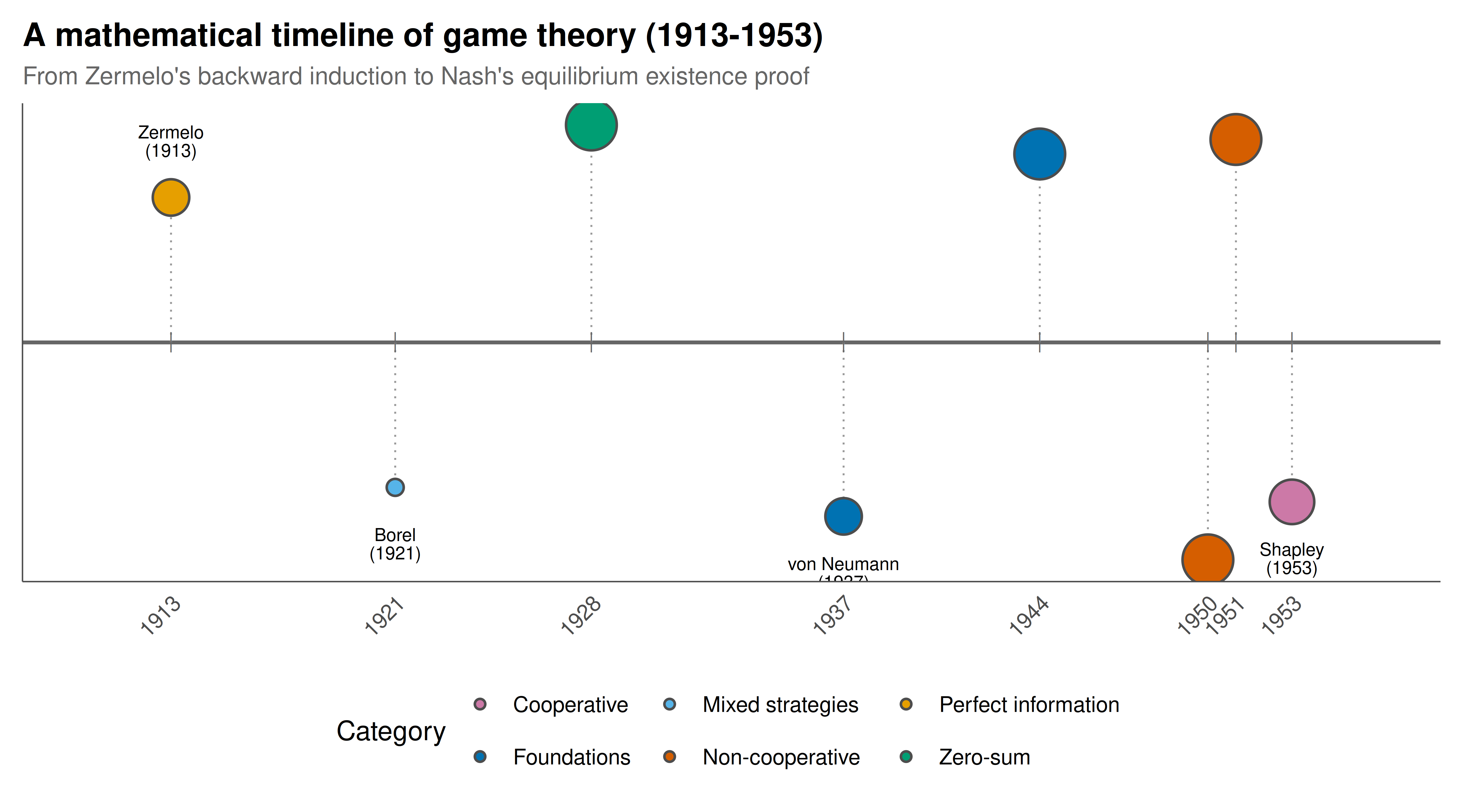
#| fig-cap: "Figure 1. Timeline of foundational game theory results (1913-1953). Circle size reflects the relative importance of each contribution. The field evolved from Zermelo's theorem on determined games through von Neumann's minimax theorem for zero-sum games to Nash's general equilibrium existence proof for all finite games. Colour indicates the mathematical category of each contribution. Okabe-Ito palette."
#| dev: [png, pdf]
#| fig-width: 9
#| fig-height: 5
#| dpi: 300
milestones <- milestones |>
  mutate(y_pos = c(1, -1, 1.5, -1.2, 1.3, -1.5, 1.4, -1.1))

p_timeline <- ggplot(milestones, aes(x = year, y = y_pos)) +
  # Timeline axis
  geom_hline(yintercept = 0, color = "grey40", linewidth = 0.8) +
  geom_segment(aes(xend = year, y = 0, yend = y_pos),
               color = "grey60", linewidth = 0.4, linetype = "dotted") +
  # Milestone points
  geom_point(aes(size = importance, fill = category),
             shape = 21, stroke = 0.8, color = "grey30") +
  # Labels
  geom_text(aes(label = paste0(author, "\n(", year, ")")),
            size = 2.8, vjust = ifelse(milestones$y_pos > 0, -1.3, 2.3),
            lineheight = 0.85) +
  # Year markers on axis
  geom_point(aes(y = 0), shape = "|", size = 3, color = "grey40") +
  scale_fill_manual(
    values = c("Perfect information" = okabe_ito[1],
               "Mixed strategies" = okabe_ito[2],
               "Zero-sum" = okabe_ito[3],
               "Foundations" = okabe_ito[5],
               "Non-cooperative" = okabe_ito[6],
               "Cooperative" = okabe_ito[7]),
    name = "Category"
  ) +
  scale_size_continuous(range = c(3, 10), guide = "none") +
  scale_x_continuous(breaks = milestones$year,
                     limits = c(1910, 1956)) +
  labs(
    title = "A mathematical timeline of game theory (1913-1953)",
    subtitle = "From Zermelo's backward induction to Nash's equilibrium existence proof",
    x = NULL, y = NULL
  ) +
  theme_publication() +
  theme(axis.text.y = element_blank(),
        axis.ticks.y = element_blank(),
        panel.grid.major.y = element_blank(),
        panel.grid.major.x = element_blank(),
        axis.text.x = element_text(angle = 45, hjust = 1))

p_timeline
```
## Interactive figure
```{r}
#| label: fig-minimax-interactive
# Interactive visualization of the minimax theorem
minimax_df <- tibble(
  p = rep(p_grid, 2),
  value = c(maximin_values, minimax_values),
  type = rep(c("Maximin (P1 maximises)", "Minimax (P2 minimises)"),
             each = length(p_grid))
) |>
  mutate(text = paste0("Strategy: p = ", round(p, 2),
                       "\nValue: ", round(value, 3),
                       "\n", type))

p_mm <- ggplot(minimax_df, aes(x = p, y = value, color = type, text = text)) +
  geom_line(linewidth = 1) +
  geom_hline(yintercept = 0, linetype = "dashed", color = "grey50") +
  geom_vline(xintercept = 0.5, linetype = "dotted", color = "grey50") +
  annotate("point", x = 0.5, y = 0, size = 4, shape = 18,
           color = okabe_ito[6]) +
  scale_color_manual(
    values = c("Maximin (P1 maximises)" = okabe_ito[1],
               "Minimax (P2 minimises)" = okabe_ito[3]),
    name = NULL
  ) +
  labs(
    title = "Von Neumann's minimax theorem — matching pennies",
    subtitle = "Maximin and minimax curves meet at the saddle point (p = 0.5, v = 0)",
    x = "Player 1's probability of Heads (p)",
    y = "Game value"
  ) +
  theme_publication()

ggplotly(p_mm, tooltip = "text") |>
  config(displaylogo = FALSE,
         modeBarButtonsToRemove = c("select2d", "lasso2d"))
```
## Interpretation
The timeline reveals how game theory progressed through a series of increasing generalisations. Zermelo's 1913 result was specific to games of perfect information — chess-like games where all moves are observable and there is no randomness. Borel explored mixed strategies but could only verify the minimax property for games with at most five pure strategies, and he doubted it would hold generally. Von Neumann's 1928 minimax theorem was the first great breakthrough: it proved that in any two-person zero-sum game, randomisation (mixed strategies) guarantees the existence of a saddle point where maximin equals minimax. The proof drew on topology (Brouwer's fixed point theorem), connecting game theory to deep mathematics. The 1944 book with Morgenstern gave the field its conceptual foundations — the extensive and normal form representations, the expected utility axioms, and the characteristic function for cooperative games — but the theory remained limited to zero-sum or cooperative settings. Nash's contribution was decisive precisely because it removed these restrictions. His 27-page PhD thesis showed that every finite game (any number of players, any payoff structure) has at least one equilibrium in mixed strategies. The proof's elegance — constructing a continuous self-map on the strategy space whose fixed points are equilibria — made it immediately influential. Remarkably, Nash was only 22 when he submitted the one-page PNAS note in 1950 and 23 when the full proof appeared in the Annals of Mathematics. Shapley's 1953 value for cooperative games completed the classical foundations, giving the field both non-cooperative (Nash) and cooperative (Shapley) solution concepts that remain central to this day.
## Extensions & related tutorials
- [Zero-sum games and the minimax theorem](../../foundations/zero-sum-minimax-theorem/) — detailed treatment of von Neumann's result.
- [Nash equilibrium: existence and computation](../../foundations/nash-equilibrium-mixed/) — Nash's theorem in depth.
- [The Shapley value](../../cooperative-gt/shapley-value/) — Shapley's 1953 fair division concept.
- [Backward induction and subgame perfection](../../foundations/backward-induction/) — Zermelo's idea formalised.
- [Matching pennies](../../classical-games/matching-pennies/) — the canonical zero-sum game.
## References
::: {#refs}
:::