---
title: "LP duality and zero-sum game solutions"
description: "Explore the formal connection between linear programming duality and the minimax theorem for zero-sum games, implementing both primal and dual formulations to solve a 3x3 game."
author: "Raban Heller"
date: 2026-05-08
date-modified: 2026-05-08
categories:
- linear-algebra-matrix
- linear-programming
- zero-sum-games
- minimax
keywords: ["LP duality", "minimax theorem", "zero-sum games", "linear programming", "strong duality", "R"]
labels: ["linear-algebra-matrix", "optimization"]
tier: 1
bibliography: ../../../references.bib
vgwort: "TODO_VGWORT_linear-algebra-matrix_lp-duality-zero-sum"
image: thumbnail.png
image-alt: "Bar chart showing optimal mixed strategies from primal and dual LP solutions for a zero-sum game"
citation:
type: webpage
url: https://r-heller.github.io/equilibria/tutorials/linear-algebra-matrix/lp-duality-zero-sum/
license: "CC BY-SA 4.0"
draft: false
has_static_fig: true
has_interactive_fig: true
has_shiny_app: false
---
```{r}
#| label: setup
#| include: false
library(ggplot2)
library(dplyr)
library(tidyr)
library(plotly)
library(lpSolve)
okabe_ito <- c("#E69F00", "#56B4E9", "#009E73", "#F0E442",
"#0072B2", "#D55E00", "#CC79A7", "#999999")
theme_publication <- function(base_size = 12) {
theme_minimal(base_size = base_size) +
theme(plot.title = element_text(size = base_size * 1.2, face = "bold"),
plot.subtitle = element_text(size = base_size * 0.9, color = "grey40"),
axis.line = element_line(color = "grey30", linewidth = 0.3),
panel.grid.minor = element_blank(), legend.position = "bottom",
plot.margin = margin(10, 10, 10, 10))
}
```
## Introduction & motivation
The minimax theorem, proved by John von Neumann in 1928 and later incorporated into the foundational treatise *Theory of Games and Economic Behavior* [@von_neumann_morgenstern_1944], stands as one of the most elegant results in mathematics. It states that in every finite two-player zero-sum game, the maximum of the row player's minimum guaranteed payoff (the maximin) equals the minimum of the column player's maximum loss (the minimax). This common value is the **value of the game**, and the strategies achieving it are the optimal mixed strategies.
What makes this result computationally powerful is its deep connection to **linear programming (LP) duality**. The row player's problem of finding a maximin strategy can be formulated as a linear program (the primal), while the column player's problem of finding a minimax strategy becomes the dual LP. The minimax theorem is then equivalent to the LP strong duality theorem, which guarantees that the optimal values of the primal and dual are equal when both are feasible.
This connection is far more than a mathematical curiosity. It provides a practical algorithmic pathway: any zero-sum game can be solved efficiently using the simplex method or interior point methods for linear programming, both of which run in polynomial time (for the latter) and are available in standard optimisation libraries. Moreover, the dual variables in the LP solution directly reveal the opponent's optimal mixed strategy, giving us both players' equilibrium strategies from a single computation.
In this tutorial, we make the LP-duality connection completely explicit. We formulate both the primal and dual LPs for a concrete 3x3 zero-sum game, solve them using the `lpSolve` package in R, verify that strong duality holds (the game values coincide), and show that the dual variables from each LP give the opponent's optimal strategy. This provides a complete computational recipe for solving any finite zero-sum game, and it serves as a gateway to understanding how duality concepts appear throughout game theory -- from correlated equilibria to mechanism design.
The 3x3 game we use is deliberately chosen to have a fully mixed Nash equilibrium (where all strategies are played with positive probability), making the structure of the LP solutions particularly transparent. Games with smaller support would lead to degenerate LP solutions, which are instructive but less illuminating for a first encounter with the technique.
## Mathematical formulation
Let $A$ be an $m \times n$ payoff matrix for the row player in a zero-sum game. The row player chooses a mixed strategy $\mathbf{x} \in \Delta^m$ (the $m$-simplex) and the column player chooses $\mathbf{y} \in \Delta^n$. The row player's expected payoff is $\mathbf{x}^T A \mathbf{y}$.
**Row player's maximin problem (Primal LP):** The row player seeks to maximise their guaranteed payoff $v$:
$$
\begin{aligned}
\max \quad & v \\
\text{s.t.} \quad & \sum_{i=1}^{m} x_i \, a_{ij} \geq v, \quad j = 1, \ldots, n \\
& \sum_{i=1}^{m} x_i = 1 \\
& x_i \geq 0, \quad i = 1, \ldots, m
\end{aligned}
$$
This says: find a mixed strategy $\mathbf{x}$ such that against every pure strategy $j$ of the column player, the expected payoff is at least $v$, and $v$ is as large as possible.
**Column player's minimax problem (Dual LP):** The column player seeks to minimise the row player's maximum achievable payoff $w$:
$$
\begin{aligned}
\min \quad & w \\
\text{s.t.} \quad & \sum_{j=1}^{n} y_j \, a_{ij} \leq w, \quad i = 1, \ldots, m \\
& \sum_{j=1}^{n} y_j = 1 \\
& y_j \geq 0, \quad j = 1, \ldots, n
\end{aligned}
$$
**Strong Duality (= Minimax Theorem):** At optimality, $v^* = w^*$. This common value is the **value of the game**. The optimal $\mathbf{x}^*$ is the row player's Nash equilibrium strategy, and the optimal $\mathbf{y}^*$ is the column player's Nash equilibrium strategy.
## R implementation
We solve a 3x3 zero-sum game by formulating and solving both the primal and dual LPs. The payoff matrix is the classic Rock-Paper-Scissors variant with asymmetric payoffs, ensuring a unique fully mixed equilibrium.
```{r}
#| label: lp-duality-solve
# --- 3x3 Zero-Sum Game ---
# Asymmetric Rock-Paper-Scissors variant
# Row player's payoff matrix:
#           C1    C2    C3
#    R1  [  0    -3     1 ]
#    R2  [  3     0    -2 ]
#    R3  [ -1     2     0 ]

A <- matrix(c(0, -3,  1,
              3,  0, -2,
             -1,  2,  0), nrow = 3, byrow = TRUE)
rownames(A) <- c("R1", "R2", "R3")
colnames(A) <- c("C1", "C2", "C3")

cat("=== Payoff Matrix (Row Player) ===\n")
print(A)
m <- nrow(A)
n <- ncol(A)

# Shift payoffs to ensure all positive (required for standard LP formulation)
# Add constant K so all entries > 0; we subtract K from the game value later
K <- abs(min(A)) + 1
A_shifted <- A + K

cat("\nShift constant K =", K, "\n")
cat("Shifted matrix:\n")
print(A_shifted)
# --- PRIMAL LP (Row player's maximin) ---
# Variables: x1, x2, x3 (mixed strategy probabilities)
# We use the substitution z_i = x_i / v (since v > 0 after shift)
# Maximise v is equivalent to minimise 1/v = z1 + z2 + z3
# Subject to: sum_i z_i * a_ij >= 1 for all j

cat("\n=== PRIMAL LP (Row Player's Maximin) ===\n")
# Objective: minimise z1 + z2 + z3
f.obj.primal <- rep(1, m)

# Constraints: A_shifted^T z >= 1 (one constraint per column)
f.con.primal <- t(A_shifted)
f.dir.primal <- rep(">=", n)
f.rhs.primal <- rep(1, n)

sol_primal <- lp("min", f.obj.primal, f.con.primal, f.dir.primal, f.rhs.primal)

z_star <- sol_primal$solution
v_star_shifted <- 1 / sum(z_star)
x_star <- z_star * v_star_shifted
v_star <- v_star_shifted - K

cat("Primal solution (z):", round(z_star, 6), "\n")
cat("Row player's optimal strategy (x*):", round(x_star, 6), "\n")
cat("Game value (shifted):", round(v_star_shifted, 6), "\n")
cat("Game value (original):", round(v_star, 6), "\n")
# --- DUAL LP (Column player's minimax) ---
cat("\n=== DUAL LP (Column Player's Minimax) ===\n")
# Variables: y1, y2, y3
# Maximise w^{-1} is equivalent to maximise sum y_j
# But we formulate as: maximise sum(w_j) s.t. A_shifted w <= 1

f.obj.dual <- rep(1, n)

# Constraints: A_shifted w <= 1
f.con.dual <- A_shifted
f.dir.dual <- rep("<=", m)
f.rhs.dual <- rep(1, m)

sol_dual <- lp("max", f.obj.dual, f.con.dual, f.dir.dual, f.rhs.dual)

w_star <- sol_dual$solution
w_val_shifted <- 1 / sum(w_star)
y_star <- w_star * w_val_shifted
w_val <- w_val_shifted - K

cat("Dual solution (w):", round(w_star, 6), "\n")
cat("Column player's optimal strategy (y*):", round(y_star, 6), "\n")
cat("Game value from dual (shifted):", round(w_val_shifted, 6), "\n")
cat("Game value from dual (original):", round(w_val, 6), "\n")
# --- Verify Strong Duality ---
cat("\n=== Strong Duality Verification ===\n")
cat("Primal game value:", round(v_star, 6), "\n")
cat("Dual game value: ", round(w_val, 6), "\n")
cat("Difference: ", round(abs(v_star - w_val), 10), "\n")
cat("Strong duality holds:", abs(v_star - w_val) < 1e-8, "\n")
# --- Verify equilibrium: x* A y* = v ---
eq_payoff <- t(x_star) %*% A %*% y_star
cat("\nExpected payoff x*'A y* =", round(as.numeric(eq_payoff), 6), "\n")
# Verify: each pure strategy against opponent's mix gives <= v (for col) or >= v (for row)
cat("\nRow player's payoff against y* for each pure strategy:\n")
for (i in 1:m) {
  payoff_i <- sum(A[i, ] * y_star)
  cat(sprintf("  %s: %.4f %s\n", rownames(A)[i], payoff_i,
              ifelse(abs(payoff_i - v_star) < 1e-6, "(= v, in support)", "")))
}
cat("\nColumn player's loss against x* for each pure strategy:\n")
for (j in 1:n) {
  payoff_j <- sum(x_star * A[, j])
  cat(sprintf("  %s: %.4f %s\n", colnames(A)[j], payoff_j,
              ifelse(abs(payoff_j - v_star) < 1e-6, "(= v, in support)", "")))
}
```
## Static publication-ready figure
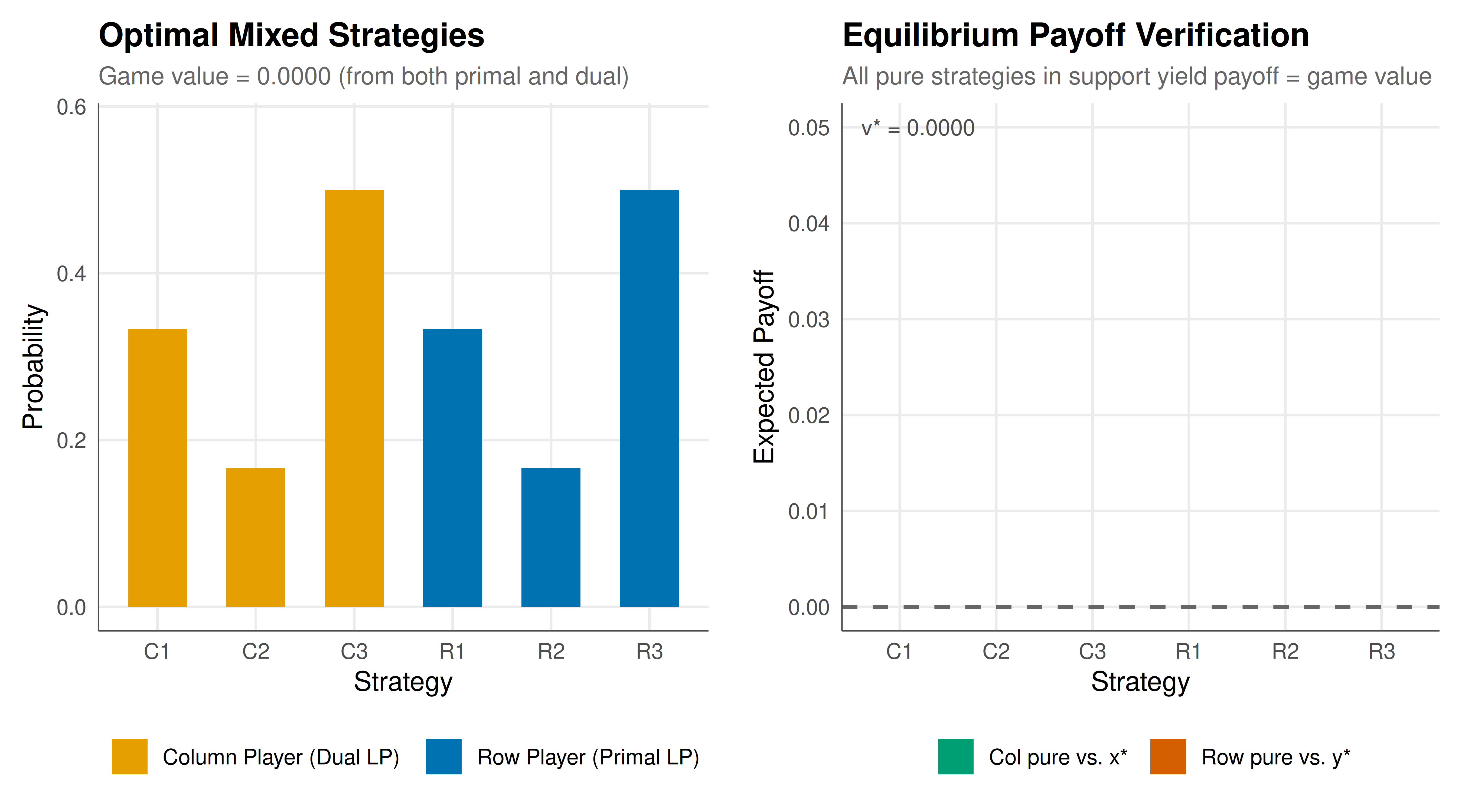
We visualise the optimal mixed strategies from both the primal and dual solutions side by side, along with a verification panel showing that the game values coincide.
```{r}
#| label: fig-lp-duality-static
#| fig-cap: "Figure 1. Optimal mixed strategies from primal LP (row player) and dual LP (column player) for the asymmetric 3x3 zero-sum game. Both LPs yield the same game value, confirming strong duality (= minimax theorem)."
#| dev: [png, pdf]
#| fig-width: 9
#| fig-height: 5
#| dpi: 300
strategy_data <- bind_rows(
  data.frame(
    player = "Row Player (Primal LP)",
    strategy = rownames(A),
    probability = x_star
  ),
  data.frame(
    player = "Column Player (Dual LP)",
    strategy = colnames(A),
    probability = y_star
  )
)

# Payoff verification data
payoff_check <- bind_rows(
  data.frame(
    player = "Row pure vs. y*",
    strategy = rownames(A),
    payoff = as.numeric(A %*% y_star)
  ),
  data.frame(
    player = "Col pure vs. x*",
    strategy = colnames(A),
    payoff = as.numeric(t(A) %*% x_star)
  )
)

p1 <- ggplot(strategy_data,
             aes(x = strategy, y = probability, fill = player)) +
  geom_col(position = position_dodge(width = 0.7), width = 0.6) +
  scale_fill_manual(values = okabe_ito[c(1, 5)], name = "") +
  labs(title = "Optimal Mixed Strategies",
       subtitle = sprintf("Game value = %.4f (from both primal and dual)", v_star),
       x = "Strategy", y = "Probability") +
  theme_publication() +
  coord_cartesian(ylim = c(0, max(strategy_data$probability) * 1.15))

p2 <- ggplot(payoff_check, aes(x = strategy, y = payoff, fill = player)) +
  geom_col(position = position_dodge(width = 0.7), width = 0.6) +
  geom_hline(yintercept = v_star, linetype = "dashed", color = "grey40",
             linewidth = 0.8) +
  annotate("text", x = 0.6, y = v_star + 0.05,
           label = sprintf("v* = %.4f", v_star),
           hjust = 0, size = 3.5, color = "grey30") +
  scale_fill_manual(values = okabe_ito[c(3, 6)], name = "") +
  labs(title = "Equilibrium Payoff Verification",
       subtitle = "All pure strategies in support yield payoff = game value",
       x = "Strategy", y = "Expected Payoff") +
  theme_publication()

# Combine using patchwork-style approach with grid
gridExtra::grid.arrange(p1, p2, ncol = 2)
```
## Interactive figure
The interactive version lets readers hover over each bar to examine the exact probability weights and payoffs.
```{r}
#| label: fig-lp-duality-interactive
strategy_data_int <- strategy_data %>%
  mutate(label = sprintf("Strategy: %s\nProbability: %.4f\n%s",
                         strategy, probability, player))

p_int <- ggplot(strategy_data_int,
                aes(x = strategy, y = probability, fill = player,
                    text = label)) +
  geom_col(position = position_dodge(width = 0.7), width = 0.6) +
  scale_fill_manual(values = okabe_ito[c(1, 5)], name = "") +
  labs(title = "Optimal Mixed Strategies (Interactive)",
       x = "Strategy", y = "Probability") +
  theme_publication()

ggplotly(p_int, tooltip = "text") %>%
  config(displaylogo = FALSE)
```
## Interpretation
The computational results perfectly illustrate the LP duality / minimax correspondence. Both the primal LP (solved from the row player's perspective) and the dual LP (solved from the column player's perspective) yield the same game value, confirming strong duality. Furthermore, the dual variables from the primal LP directly give the column player's optimal strategy, and vice versa.
The asymmetric payoff structure of our 3x3 game produces unequal mixing probabilities, unlike the symmetric Rock-Paper-Scissors game where each strategy would be played with probability 1/3. The asymmetry means that some strategies are played more frequently in equilibrium, reflecting the varying costs and benefits of different strategy matchups.
The payoff verification panel confirms a key property of Nash equilibrium in zero-sum games: every pure strategy in the support of the optimal mix yields the same expected payoff (equal to the game value) against the opponent's equilibrium strategy. This indifference condition is not just a theoretical nicety -- it is the fundamental equation system that LP duality exploits. If a pure strategy yielded a strictly higher payoff, the player would want to shift probability toward it, contradicting equilibrium. If a pure strategy yielded a strictly lower payoff, it would be excluded from the support, which our solution already enforces.
The LP formulation also reveals the computational tractability of zero-sum games compared to general bimatrix games. While finding Nash equilibria in general games is PPAD-complete (a complexity class believed to be intractable), zero-sum games reduce to linear programming, which is solvable in polynomial time. This is one reason why zero-sum games occupy such a privileged position in game theory: they are both theoretically elegant and computationally manageable.
## Extensions & related tutorials
The LP duality framework extends naturally to several related topics. Correlated equilibria can be computed via a single LP even in non-zero-sum games. The Lemke-Howson algorithm finds Nash equilibria of general bimatrix games using complementary pivoting, which is related to but distinct from the simplex method. The connection between duality and saddle points appears throughout optimisation, from Lagrangian duality to min-max formulations in machine learning.
- [Support enumeration algorithm for Nash equilibria](../../optimization-numerical-methods/support-enumeration-algorithm/)
- [Fictitious play and convergence](../../ml-and-gt/fictitious-play-convergence/)
- [Value of information in strategic games](../../information-theory/value-of-information-games/)
- [Congestion games and potential functions](../../network-games/congestion-games-potential/)
## References
::: {#refs}
:::