---
title: "Fictitious play and convergence"
description: "Implement Brown's fictitious play algorithm for 2x2 and 3x3 games, demonstrating convergence in zero-sum and potential games and the classic non-convergence cycling in Shapley's counterexample."
author: "Raban Heller"
date: 2026-05-08
date-modified: 2026-05-08
categories:
- ml-and-gt
- fictitious-play
- learning-in-games
- nash-equilibrium
keywords: ["fictitious play", "Brown", "Robinson theorem", "Shapley counterexample", "learning dynamics", "convergence", "R"]
labels: ["ml-and-gt", "learning-in-games"]
tier: 1
bibliography: ../../../references.bib
vgwort: "TODO_VGWORT_ml-and-gt_fictitious-play-convergence"
image: thumbnail.png
image-alt: "Trajectory plots showing fictitious play convergence in a zero-sum game and cycling in Shapley's counterexample"
citation:
type: webpage
url: https://r-heller.github.io/equilibria/tutorials/ml-and-gt/fictitious-play-convergence/
license: "CC BY-SA 4.0"
draft: false
has_static_fig: true
has_interactive_fig: true
has_shiny_app: false
---
```{r}
#| label: setup
#| include: false
library(ggplot2)
library(dplyr)
library(tidyr)
library(plotly)
okabe_ito <- c("#E69F00", "#56B4E9", "#009E73", "#F0E442",
"#0072B2", "#D55E00", "#CC79A7", "#999999")
theme_publication <- function(base_size = 12) {
theme_minimal(base_size = base_size) +
theme(plot.title = element_text(size = base_size * 1.2, face = "bold"),
plot.subtitle = element_text(size = base_size * 0.9, color = "grey40"),
axis.line = element_line(color = "grey30", linewidth = 0.3),
panel.grid.minor = element_blank(), legend.position = "bottom",
plot.margin = margin(10, 10, 10, 10))
}
```
## Introduction & motivation
How do players learn to play a Nash equilibrium? If each player knows the game's payoff structure but not the opponent's strategy, one natural approach is to observe the opponent's past actions and best-respond to the empirical frequency of those actions. This is the core idea behind **fictitious play**, introduced by George W. Brown in 1951 as a computational method for solving games. In fictitious play, each player maintains a count of how often the opponent has played each action, treats the resulting empirical distribution as a belief about the opponent's mixed strategy, and plays a best response to that belief at each step.
The remarkable theoretical result, proved by Julia Robinson in 1951, is that fictitious play converges to the Nash equilibrium value in every finite two-player zero-sum game. More precisely, the empirical frequencies of play converge to the set of Nash equilibria, and the time-averaged payoffs converge to the game value. This makes fictitious play one of the earliest and most natural learning algorithms for games, predating modern multi-agent reinforcement learning by decades.
Beyond zero-sum games, fictitious play also converges in several important classes of games. In **potential games** (games where players' incentives are aligned with a single global potential function), fictitious play converges because the best-response dynamics implicitly reduce the potential. In $2 \times 2$ games, convergence is guaranteed regardless of the payoff structure. In games with identical interests (where all players have the same payoff function), convergence also holds.
However, fictitious play does not converge in all games. The most famous counterexample is due to **Lloyd Shapley** (1964), who constructed a $3 \times 3$ non-zero-sum game where the empirical frequencies of play cycle indefinitely without converging to any equilibrium. In Shapley's game, the best-response dynamics trace out an orbit that never settles down, even as the cycle slows over time. This counterexample was historically important because it showed that simple adaptive learning rules cannot solve all games, motivating the development of more sophisticated learning algorithms such as smooth fictitious play, regret matching, and multiplicative weights update.
In this tutorial, we implement fictitious play from scratch, apply it to three games (a 2x2 zero-sum game where it converges, a coordination game as a potential game where it also converges, and Shapley's 3x3 counterexample where it cycles), and visualise the empirical frequency trajectories to see convergence and cycling directly.
## Mathematical formulation
Consider a two-player game with row player action set $\{1, \ldots, m\}$, column player action set $\{1, \ldots, n\}$, and payoff matrices $A$ (row player) and $B$ (column player). In a zero-sum game, $B = -A$.
**Fictitious play process:** At time $t$, let $\mathbf{c}^1_t \in \mathbb{Z}^m$ and $\mathbf{c}^2_t \in \mathbb{Z}^n$ be the cumulative counts of actions played by players 1 and 2 respectively. The empirical frequencies are:
$$
\hat{\mathbf{x}}_t = \frac{\mathbf{c}^1_t}{t}, \qquad \hat{\mathbf{y}}_t = \frac{\mathbf{c}^2_t}{t}
$$
At time $t+1$, each player best-responds to the opponent's empirical frequency:
$$
a^1_{t+1} \in \arg\max_{i} \sum_{j} a_{ij} \, \hat{y}_{t,j}, \qquad a^2_{t+1} \in \arg\max_{j} \sum_{i} b_{ij} \, \hat{x}_{t,i}
$$
Counts are updated: $c^1_{t+1, i} = c^1_{t, i} + \mathbf{1}[a^1_{t+1} = i]$ and similarly for player 2.
**Robinson's Theorem (1951):** In any finite two-player zero-sum game, the empirical frequencies $(\hat{\mathbf{x}}_t, \hat{\mathbf{y}}_t)$ converge to the set of Nash equilibria as $t \to \infty$.
**Shapley's counterexample (1964):** The bimatrix game with:
$$
A = \begin{pmatrix} 1 & 0 & 0 \\ 0 & 1 & 0 \\ 0 & 0 & 1 \end{pmatrix}, \quad
B = \begin{pmatrix} 0 & 1 & 0 \\ 0 & 0 & 1 \\ 1 & 0 & 0 \end{pmatrix}
$$
has the unique Nash equilibrium $((1/3, 1/3, 1/3), (1/3, 1/3, 1/3))$, but fictitious play from any non-equilibrium starting point cycles indefinitely, with the empirical frequencies tracing a closed orbit in the strategy simplex.
## R implementation
We implement a general fictitious play function and apply it to three games.
```{r}
#| label: fictitious-play-implementation
# General fictitious play implementation
fictitious_play <- function(A, B, n_rounds = 1000, seed = 42) {
  set.seed(seed)
  m <- nrow(A)
  n <- ncol(A)

  # Initialise: each player plays a random action

  counts_1 <- rep(0, m)  # cumulative action counts for player 1
  counts_2 <- rep(0, n)  # cumulative action counts for player 2

  # Initial actions
  a1 <- sample(1:m, 1)
  a2 <- sample(1:n, 1)
  counts_1[a1] <- 1
  counts_2[a2] <- 1

  # Storage for empirical frequencies
  history_x <- matrix(0, nrow = n_rounds, ncol = m)
  history_y <- matrix(0, nrow = n_rounds, ncol = n)
  history_x[1, ] <- counts_1
  history_y[1, ] <- counts_2

  for (t in 2:n_rounds) {
    # Empirical frequencies
    freq_2 <- counts_2 / sum(counts_2)
    freq_1 <- counts_1 / sum(counts_1)

    # Best responses
    payoffs_1 <- A %*% freq_2
    payoffs_2 <- t(B) %*% freq_1

    a1 <- which.max(payoffs_1)
    a2 <- which.max(payoffs_2)

    counts_1[a1] <- counts_1[a1] + 1
    counts_2[a2] <- counts_2[a2] + 1

    history_x[t, ] <- counts_1 / sum(counts_1)
    history_y[t, ] <- counts_2 / sum(counts_2)
  }

  list(x = history_x, y = history_y)
}

# === Game 1: 2x2 Zero-Sum (Matching Pennies) ===
cat("=== Game 1: Matching Pennies (Zero-Sum) ===\n")
A1 <- matrix(c(1, -1, -1, 1), nrow = 2, byrow = TRUE)
B1 <- -A1
cat("Payoff matrix A:\n"); print(A1)
cat("NE: (0.5, 0.5) for both players\n\n")
fp1 <- fictitious_play(A1, B1, n_rounds = 500)
cat("After 500 rounds:\n")
cat(" Player 1 empirical freq:", round(fp1$x[500, ], 4), "\n")
cat(" Player 2 empirical freq:", round(fp1$y[500, ], 4), "\n")
# === Game 2: Coordination Game (Potential Game) ===
cat("\n=== Game 2: Coordination Game (Potential Game) ===\n")
A2 <- matrix(c(2, 0, 0, 1), nrow = 2, byrow = TRUE)
B2 <- A2  # identical interests
cat("Payoff matrix (same for both):\n"); print(A2)
cat("Pure NE: (1,1) and (2,2)\n\n")
fp2 <- fictitious_play(A2, B2, n_rounds = 500)
cat("After 500 rounds:\n")
cat(" Player 1 empirical freq:", round(fp2$x[500, ], 4), "\n")
cat(" Player 2 empirical freq:", round(fp2$y[500, ], 4), "\n")
# === Game 3: Shapley's Counterexample ===
cat("\n=== Game 3: Shapley's Counterexample (Non-Convergence) ===\n")
A3 <- matrix(c(1, 0, 0,
               0, 1, 0,
               0, 0, 1), nrow = 3, byrow = TRUE)
B3 <- matrix(c(0, 1, 0,
               0, 0, 1,
               1, 0, 0), nrow = 3, byrow = TRUE)
cat("A (Row player):\n"); print(A3)
cat("B (Column player):\n"); print(B3)
cat("Unique NE: (1/3, 1/3, 1/3) for both\n\n")
fp3 <- fictitious_play(A3, B3, n_rounds = 2000)
cat("After 2000 rounds:\n")
cat(" Player 1 empirical freq:", round(fp3$x[2000, ], 4), "\n")
cat(" Player 2 empirical freq:", round(fp3$y[2000, ], 4), "\n")
# Check distance from NE
ne_3 <- rep(1/3, 3)
dist_from_ne <- sqrt(sum((fp3$x[2000, ] - ne_3)^2))
cat("  L2 distance from NE:", round(dist_from_ne, 4), "\n")
cat(" (Non-zero distance indicates cycling / non-convergence)\n")
```
## Static publication-ready figure
We create a multi-panel figure showing the empirical frequency trajectories for all three games, making convergence (or lack thereof) visually apparent.
```{r}
#| label: fig-fictitious-play-static
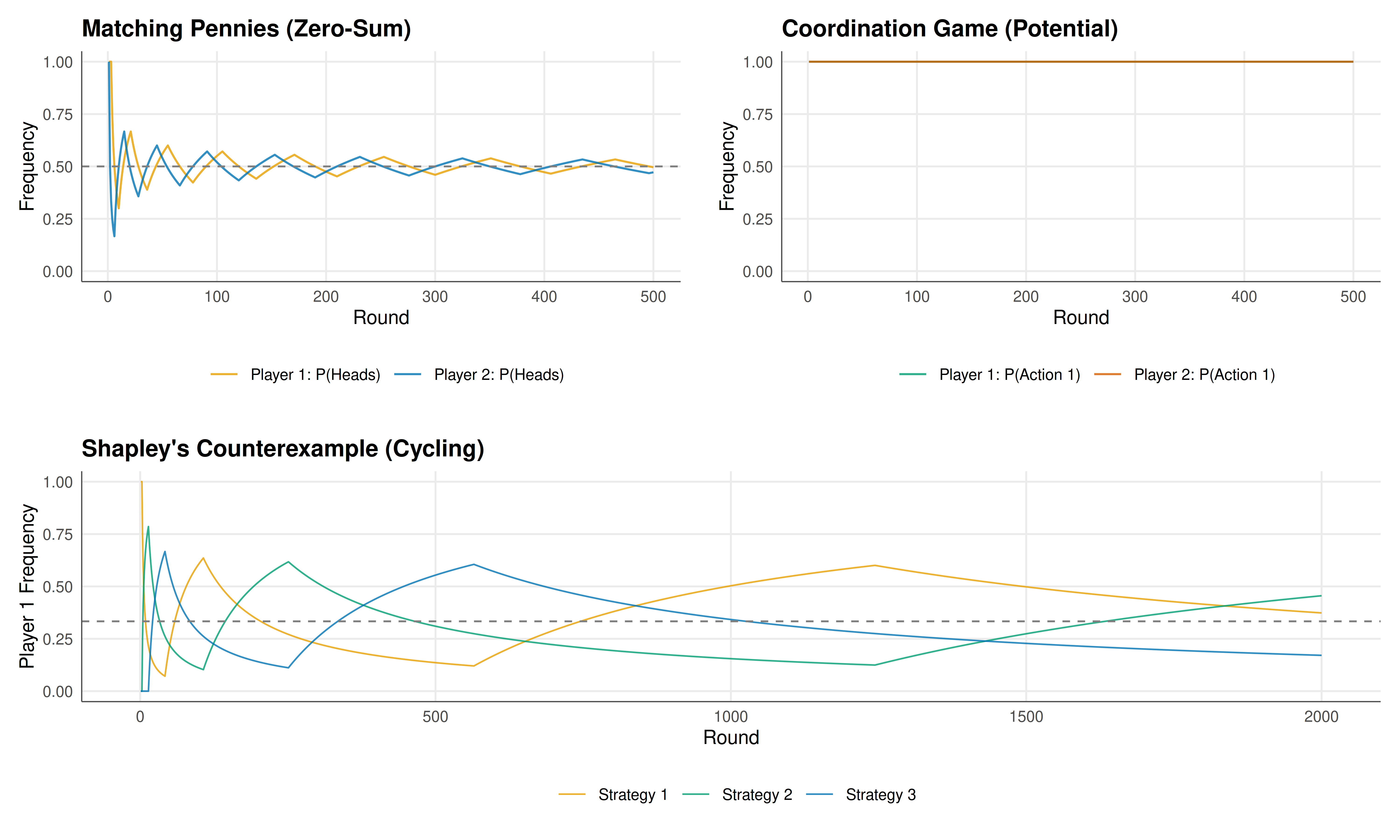
#| fig-cap: "Figure 1. Fictitious play empirical frequency trajectories. Top-left: Matching Pennies converges to (0.5, 0.5). Top-right: Coordination game converges to a pure equilibrium. Bottom: Shapley's counterexample cycles around (1/3, 1/3, 1/3) without converging."
#| dev: [png, pdf]
#| fig-width: 10
#| fig-height: 6
#| dpi: 300
# Prepare data for Game 1 (zero-sum convergence)
df1 <- data.frame(
  t = 1:500,
  p1 = fp1$x[1:500, 1],
  p2 = fp1$y[1:500, 1]
) %>%
  pivot_longer(cols = c(p1, p2),
               names_to = "player",
               values_to = "freq_action1") %>%
  mutate(player = ifelse(player == "p1", "Player 1: P(Heads)",
                         "Player 2: P(Heads)"),
         game = "Matching Pennies (Zero-Sum)")

# Prepare data for Game 2 (potential game convergence)
df2 <- data.frame(
  t = 1:500,
  p1 = fp2$x[1:500, 1],
  p2 = fp2$y[1:500, 1]
) %>%
  pivot_longer(cols = c(p1, p2),
               names_to = "player",
               values_to = "freq_action1") %>%
  mutate(player = ifelse(player == "p1", "Player 1: P(Action 1)",
                         "Player 2: P(Action 1)"),
         game = "Coordination (Potential Game)")

# Prepare data for Game 3 (Shapley cycling) - show all 3 strategies for player 1
df3 <- data.frame(
  t = rep(1:2000, 3),
  strategy = rep(c("Strategy 1", "Strategy 2", "Strategy 3"), each = 2000),
  freq = c(fp3$x[1:2000, 1], fp3$x[1:2000, 2], fp3$x[1:2000, 3]),
  game = "Shapley's Counterexample (Player 1)"
)

p_g1 <- ggplot(df1, aes(x = t, y = freq_action1, color = player)) +
  geom_line(linewidth = 0.5, alpha = 0.8) +
  geom_hline(yintercept = 0.5, linetype = "dashed", color = "grey50") +
  scale_color_manual(values = okabe_ito[c(1, 5)], name = "") +
  labs(title = "Matching Pennies (Zero-Sum)", x = "Round", y = "Frequency") +
  theme_publication(base_size = 10) +
  coord_cartesian(ylim = c(0, 1))

p_g2 <- ggplot(df2, aes(x = t, y = freq_action1, color = player)) +
  geom_line(linewidth = 0.5, alpha = 0.8) +
  scale_color_manual(values = okabe_ito[c(3, 6)], name = "") +
  labs(title = "Coordination Game (Potential)", x = "Round", y = "Frequency") +
  theme_publication(base_size = 10) +
  coord_cartesian(ylim = c(0, 1))

p_g3 <- ggplot(df3, aes(x = t, y = freq, color = strategy)) +
  geom_line(linewidth = 0.4, alpha = 0.8) +
  geom_hline(yintercept = 1/3, linetype = "dashed", color = "grey50") +
  scale_color_manual(values = okabe_ito[c(1, 3, 5)], name = "") +
  labs(title = "Shapley's Counterexample (Cycling)",
       x = "Round", y = "Player 1 Frequency") +
  theme_publication(base_size = 10)

gridExtra::grid.arrange(p_g1, p_g2, p_g3, ncol = 2,
                        layout_matrix = rbind(c(1, 2), c(3, 3)))
```
## Interactive figure
The interactive figure focuses on Shapley's counterexample, plotting the trajectory in 2D simplex coordinates (since the three frequencies sum to 1, we only need two coordinates). This makes the cycling pattern clearly visible.
```{r}
#| label: fig-fictitious-play-interactive
# Plot Shapley's counterexample as trajectory in 2D simplex
# Use coordinates (x1, x2) since x3 = 1 - x1 - x2

df_simplex <- data.frame(
  x1 = fp3$x[1:2000, 1],
  x2 = fp3$x[1:2000, 2],
  t = 1:2000
) %>%
  mutate(label = sprintf("Round: %d\nP(S1): %.3f\nP(S2): %.3f\nP(S3): %.3f",
                         t, x1, x2, 1 - x1 - x2))

p_simplex <- ggplot(df_simplex, aes(x = x1, y = x2, color = t, text = label)) +
  geom_path(linewidth = 0.4, alpha = 0.7) +
  geom_point(data = data.frame(x1 = 1/3, x2 = 1/3),
             aes(x = x1, y = x2), color = "red", size = 3,
             inherit.aes = FALSE) +
  scale_color_gradient(low = okabe_ito[5], high = okabe_ito[6],
                       name = "Round") +
  labs(
    title = "Shapley's Counterexample: Cycling in the Simplex",
    subtitle = "Player 1's empirical frequencies orbit the NE (red dot) without converging",
    x = "P(Strategy 1)", y = "P(Strategy 2)"
  ) +
  theme_publication() +
  coord_fixed()

ggplotly(p_simplex, tooltip = "text") %>%
  config(displaylogo = FALSE)
```
## Interpretation
The three examples cleanly illustrate the boundaries of fictitious play as a learning algorithm. In the Matching Pennies game (a prototypical zero-sum game), fictitious play exhibits the characteristic oscillating-but-converging behaviour predicted by Robinson's theorem. The empirical frequencies swing back and forth around the Nash equilibrium of (0.5, 0.5), with the amplitude of oscillations shrinking over time at a rate proportional to $1/t$. After 500 rounds, the frequencies are very close to the equilibrium, confirming convergence.
In the coordination game, fictitious play rapidly locks into one of the two pure Nash equilibria. Because both players prefer to coordinate on the same action, the initial actions create an asymmetry that the best-response dynamics amplify. Once one action accumulates a slight lead in the empirical counts, the best-response mechanism reinforces it, and the system converges to a pure equilibrium. This illustrates the general result that fictitious play converges in potential games: since best-response dynamics reduce the potential function, the process must converge to a local (hence global, in finite games) minimum of the potential.
Shapley's counterexample reveals a fundamental limitation. Despite the unique Nash equilibrium at (1/3, 1/3, 1/3), the empirical frequencies orbit around it in a characteristic cycle. The payoff structure creates a "rock-paper-scissors" dynamic: when the opponent is playing Strategy 1 frequently, the best response is Strategy 1 for the row player (matching) but Strategy 2 for the column player (mismatching), creating a delayed pursuit pattern. The orbit never collapses to the equilibrium because the best-response dynamics always overshoot. The simplex plot makes this cycling pattern vivid, showing the empirical frequency tracing an orbit that never reaches the red equilibrium point.
These results have significant implications for multi-agent learning. The convergence guarantees in zero-sum and potential games provide a strong foundation for using fictitious play (and its variants) in those settings. However, the non-convergence in general games motivates the development of algorithms with stronger convergence guarantees, such as regret matching (which converges to coarse correlated equilibria in all games) and multiplicative weights update (which achieves no-regret guarantees).
## Extensions & related tutorials
Fictitious play is the starting point for a rich family of learning algorithms in games. Smooth fictitious play adds noise to the best-response function (using a logit or other quantal response), which can restore convergence in some cases. Regret-based learning algorithms generalise the idea but provide guarantees for broader game classes. The connection between learning dynamics and evolutionary game theory is deep: the replicator dynamic can be viewed as a continuous-time limit of certain learning processes.
- [LP duality and zero-sum game solutions](../../linear-algebra-matrix/lp-duality-zero-sum/)
- [Congestion games and potential functions](../../network-games/congestion-games-potential/)
- [Support enumeration algorithm for Nash equilibria](../../optimization-numerical-methods/support-enumeration-algorithm/)
- [Value of information in strategic games](../../information-theory/value-of-information-games/)
- [Diffusion and cascades on networks](../../network-science/diffusion-cascades-networks/)
## References
::: {#refs}
:::