---
title: "Congestion games and potential functions"
description: "Implement Rosenthal's congestion games with Monderer-Shapley potential functions, demonstrate the existence of pure Nash equilibria, and visualise Braess's paradox in a traffic network."
author: "Raban Heller"
date: 2026-05-08
date-modified: 2026-05-08
categories:
- network-games
- congestion-games
- potential-games
- braess-paradox
keywords: ["congestion games", "Rosenthal", "potential function", "Monderer-Shapley", "Braess paradox", "pure Nash equilibrium", "R"]
labels: ["network-games", "potential-games"]
tier: 1
bibliography: ../../../references.bib
vgwort: "TODO_VGWORT_network-games_congestion-games-potential"
image: thumbnail.png
image-alt: "Network diagram and bar chart illustrating Braess's paradox where adding a road increases travel time for all drivers"
citation:
type: webpage
url: https://r-heller.github.io/equilibria/tutorials/network-games/congestion-games-potential/
license: "CC BY-SA 4.0"
draft: false
has_static_fig: true
has_interactive_fig: true
has_shiny_app: false
---
```{r}
#| label: setup
#| include: false
library(ggplot2)
library(dplyr)
library(tidyr)
library(plotly)
okabe_ito <- c("#E69F00", "#56B4E9", "#009E73", "#F0E442",
"#0072B2", "#D55E00", "#CC79A7", "#999999")
theme_publication <- function(base_size = 12) {
theme_minimal(base_size = base_size) +
theme(plot.title = element_text(size = base_size * 1.2, face = "bold"),
plot.subtitle = element_text(size = base_size * 0.9, color = "grey40"),
axis.line = element_line(color = "grey30", linewidth = 0.3),
panel.grid.minor = element_blank(), legend.position = "bottom",
plot.margin = margin(10, 10, 10, 10))
}
```
## Introduction & motivation
Every morning, millions of commuters face the same problem: which route to take to work? Each driver's travel time depends not only on the roads they choose but on how many other drivers are on the same roads. This is the essence of a **congestion game**, a class of games formalised by Robert Rosenthal in 1973 where players share a common set of resources and the cost of each resource depends on how many players use it. Congestion games model not only traffic but also network routing, server load balancing, frequency allocation in telecommunications, and many other settings where shared resources become crowded.
The theoretical importance of congestion games comes from two landmark results. First, Rosenthal proved that every congestion game possesses at least one **pure-strategy Nash equilibrium**. This is a strong result because many games (such as Matching Pennies) have no pure Nash equilibrium at all. The proof is constructive: Rosenthal defined a function over the strategy profiles -- now called the **Rosenthal potential** -- that decreases whenever any player switches to a lower-cost strategy. Since the potential takes finitely many values, the best-response improvement process must terminate at a pure Nash equilibrium.
Second, Monderer and Shapley (1996) showed that the class of congestion games is essentially equivalent to the class of **potential games** -- games where a single real-valued function captures every player's incentive to deviate. Formally, a game is a potential game if there exists a function $\Phi$ such that whenever a single player changes their strategy, the change in $\Phi$ equals the change in that player's payoff. Monderer and Shapley proved that every congestion game is a potential game (with Rosenthal's potential serving as the exact potential) and that every finite potential game is isomorphic to a congestion game.
One of the most striking implications of congestion games is **Braess's paradox** (1968). Dietrich Braess discovered that in a traffic network, adding a new road can actually **increase** the travel time for every driver at equilibrium. This counterintuitive result arises because the new road changes the equilibrium flow pattern: drivers rush to use the new shortcut, overloading previously efficient routes. The paradox has been observed in real traffic networks (most famously when closing 42nd Street in New York City actually reduced congestion) and has deep implications for network design and urban planning.
In this tutorial, we implement a simple congestion game on a traffic network, demonstrate the computation of Rosenthal's potential, show how best-response dynamics converge to a pure Nash equilibrium, and then construct and visualise Braess's paradox. The implementation uses a 4-node network where 100 drivers choose between routes from origin to destination, with linear congestion cost functions on each edge.
## Mathematical formulation
A **congestion game** is defined by a tuple $\Gamma = (N, E, (S_i)_{i \in N}, (c_e)_{e \in E})$ where:
- $N = \{1, \ldots, n\}$ is the set of players
- $E = \{e_1, \ldots, e_m\}$ is the set of resources (edges/roads)
- $S_i \subseteq 2^E$ is player $i$'s strategy set (subsets of resources)
- $c_e : \{1, \ldots, n\} \to \mathbb{R}$ is the cost function for resource $e$, depending on the number of users
Given a strategy profile $\mathbf{s} = (s_1, \ldots, s_n)$, the congestion on resource $e$ is $n_e(\mathbf{s}) = |\{i : e \in s_i\}|$. Player $i$'s cost is:
$$
C_i(\mathbf{s}) = \sum_{e \in s_i} c_e(n_e(\mathbf{s}))
$$
**Rosenthal's potential function** is defined as:
$$
\Phi(\mathbf{s}) = \sum_{e \in E} \sum_{k=1}^{n_e(\mathbf{s})} c_e(k)
$$
**Key property:** For any player $i$ switching from strategy $s_i$ to $s_i'$ (while others stay fixed):
$$
\Phi(s_i', \mathbf{s}_{-i}) - \Phi(\mathbf{s}) = C_i(s_i', \mathbf{s}_{-i}) - C_i(\mathbf{s})
$$
This means the potential tracks every player's improvement exactly. Since $\Phi$ has finitely many values, any sequence of improving deviations must terminate, proving existence of a pure Nash equilibrium.
**Braess's paradox setup:** Consider a network with nodes $\{O, A, B, D\}$ and edges with linear cost functions $c_e(x) = a_e \cdot x + b_e$, where $x$ is the number of users. Without the shortcut edge $A \to B$, drivers choose between route $O \to A \to D$ and $O \to B \to D$. Adding the edge $A \to B$ (with very low cost) can increase the equilibrium cost for all.
## R implementation
We model the Braess's paradox network with 100 drivers choosing among routes, and compare equilibrium outcomes with and without the shortcut edge.
```{r}
#| label: congestion-game-implementation
# === Braess's Paradox Network ===
# Network: O -> A -> D (route 1: "top")
#          O -> B -> D (route 2: "bottom")
#          O -> A -> B -> D (route 3: "shortcut", only available with new road)

# Cost functions (linear): c(x) = a*x + b where x = number of users
# Edge costs:
#   O->A: c(x) = x/100         (congestion-sensitive)
#   A->D: c(x) = 1             (constant: highway)
#   O->B: c(x) = 1             (constant: highway)
#   B->D: c(x) = x/100         (congestion-sensitive)
#   A->B: c(x) = 0             (free shortcut, when available)

n_drivers <- 100

# --- Without shortcut (2 routes) ---
# Route 1 (Top): O->A, A->D  cost = x_top/100 + 1
# Route 2 (Bot): O->B, B->D  cost = 1 + x_bot/100
# At equilibrium: costs must be equal (or all on one route)
# x_top/100 + 1 = 1 + x_bot/100
# x_top = x_bot = 50

cat("=== Network WITHOUT Shortcut (A->B) ===\n")
cat("Route Top (O->A->D): cost = x_top/100 + 1\n")
cat("Route Bot (O->B->D): cost = 1 + x_bot/100\n\n")
x_top_no <- 50
x_bot_no <- 50
cost_top_no <- x_top_no / 100 + 1
cost_bot_no <- 1 + x_bot_no / 100

cat("Equilibrium: x_top =", x_top_no, ", x_bot =", x_bot_no, "\n")
cat("Cost per driver:", cost_top_no, "\n")
# Compute potential without shortcut
potential_no <- function(x_top) {
  x_bot <- n_drivers - x_top
  # Potential = sum over edges of sum_{k=1}^{n_e} c_e(k)
  # O->A: sum_{k=1}^{x_top} k/100
  pot_OA <- sum((1:max(x_top, 1)) / 100) * (x_top > 0)
  if (x_top == 0) pot_OA <- 0 else pot_OA <- sum((1:x_top) / 100)
  # A->D: sum_{k=1}^{x_top} 1
  pot_AD <- x_top * 1
  # O->B: sum_{k=1}^{x_bot} 1
  pot_OB <- x_bot * 1
  # B->D: sum_{k=1}^{x_bot} k/100
  if (x_bot == 0) pot_BD <- 0 else pot_BD <- sum((1:x_bot) / 100)
  pot_OA + pot_AD + pot_OB + pot_BD
}

cat("Rosenthal potential at equilibrium:", potential_no(50), "\n\n")
# --- With shortcut (3 routes) ---
# Route 1 (Top): O->A, A->D  cost = (x_top + x_short)/100 + 1
# Route 2 (Bot): O->B, B->D  cost = 1 + (x_bot + x_short)/100
# Route 3 (Shortcut): O->A, A->B, B->D  cost = (x_top + x_short)/100 + 0 + (x_bot + x_short)/100
# Note: x on O->A = x_top + x_short, x on B->D = x_bot + x_short

cat("=== Network WITH Shortcut (A->B, cost = 0) ===\n")
cat("Route Top: cost = n_OA/100 + 1\n")
cat("Route Bot: cost = 1 + n_BD/100\n")
cat("Route Shortcut: cost = n_OA/100 + 0 + n_BD/100\n")
cat(" where n_OA = x_top + x_short, n_BD = x_bot + x_short\n\n")
# Find equilibrium by exhaustive search over integer allocations
best_cost <- Inf
best_alloc <- NULL

for (x_top in 0:n_drivers) {
  for (x_short in 0:(n_drivers - x_top)) {
    x_bot <- n_drivers - x_top - x_short
    if (x_bot < 0) next

    n_OA <- x_top + x_short
    n_AD <- x_top
    n_OB <- x_bot
    n_BD <- x_bot + x_short
    n_AB <- x_short

    cost_route_top <- n_OA / 100 + 1
    cost_route_bot <- 1 + n_BD / 100
    cost_route_short <- n_OA / 100 + 0 + n_BD / 100

    # Check NE conditions: no driver wants to switch
    # A route in use must have cost <= all alternative routes
    is_ne <- TRUE
    costs <- c(cost_route_top, cost_route_bot, cost_route_short)
    flows <- c(x_top, x_bot, x_short)
    min_cost <- min(costs)

    for (r in 1:3) {
      if (flows[r] > 0 && costs[r] > min_cost + 0.011) {
        is_ne <- FALSE
        break
      }
    }

    if (is_ne) {
      # Check if this is a "tighter" NE (costs more equal)
      active_costs <- costs[flows > 0]
      spread <- max(active_costs) - min(active_costs)
      if (spread < best_cost) {
        best_cost <- spread
        best_alloc <- c(x_top, x_bot, x_short)
        best_costs <- costs
        best_flows <- flows
      }
    }
  }
}

cat("Equilibrium allocation:\n")
cat(" Top route:", best_alloc[1], "drivers\n")
cat(" Bottom route:", best_alloc[2], "drivers\n")
cat(" Shortcut route:", best_alloc[3], "drivers\n")
cat("Route costs:", round(best_costs, 4), "\n")
# Expected: all 100 use shortcut in the extreme case, or some mix
# With these parameters: shortcut cost = n_OA/100 + n_BD/100
# If all use shortcut: cost = 100/100 + 100/100 = 2
# If x_top = x_bot = 0, x_short = 100: cost = 1 + 1 = 2
# Vs. without shortcut: cost = 1.5
# Braess's paradox: equilibrium cost with shortcut > without shortcut

avg_cost_with <- sum(best_flows * best_costs) / n_drivers
cat("\nAverage cost with shortcut:", round(avg_cost_with, 4), "\n")
cat("Average cost without shortcut:", cost_top_no, "\n")
cat("Braess's paradox magnitude:", round(avg_cost_with - cost_top_no, 4), "\n")
```
```{r}
#| label: best-response-dynamics
# === Best-Response Dynamics Simulation ===
# Start from a random allocation and simulate best-response dynamics
# to show convergence to NE

set.seed(123)

# Without shortcut: 2 routes
simulate_brd_no_shortcut <- function(n_steps = 200) {
  # Random initial: each of 100 drivers randomly picks a route
  routes <- sample(1:2, n_drivers, replace = TRUE)
  history <- numeric(n_steps)

  for (t in 1:n_steps) {
    x_top <- sum(routes == 1)
    x_bot <- sum(routes == 2)

    cost_top <- x_top / 100 + 1
    cost_bot <- 1 + x_bot / 100
    history[t] <- mean(c(rep(cost_top, x_top), rep(cost_bot, x_bot)))

    # Random driver considers switching
    driver <- sample(1:n_drivers, 1)
    current_route <- routes[driver]
    current_cost <- ifelse(current_route == 1, cost_top, cost_bot)

    # Cost if switching (one fewer on current, one more on other)
    if (current_route == 1) {
      new_cost <- 1 + (x_bot + 1) / 100
    } else {
      new_cost <- (x_top + 1) / 100 + 1
    }

    if (new_cost < current_cost) {
      routes[driver] <- 3 - current_route  # switch
    }
  }

  data.frame(step = 1:n_steps, avg_cost = history, network = "Without Shortcut")
}

brd_no <- simulate_brd_no_shortcut(300)

cat("=== Best-Response Dynamics (Without Shortcut) ===\n")
cat("Initial avg cost:", round(brd_no$avg_cost[1], 4), "\n")
cat("Final avg cost:", round(brd_no$avg_cost[300], 4), "\n")
cat("Converged to NE cost:", round(1.5, 4), "\n")
```
## Static publication-ready figure
We visualise Braess's paradox by comparing the equilibrium costs with and without the shortcut, and show the best-response dynamics converging to equilibrium.
```{r}
#| label: fig-braess-static
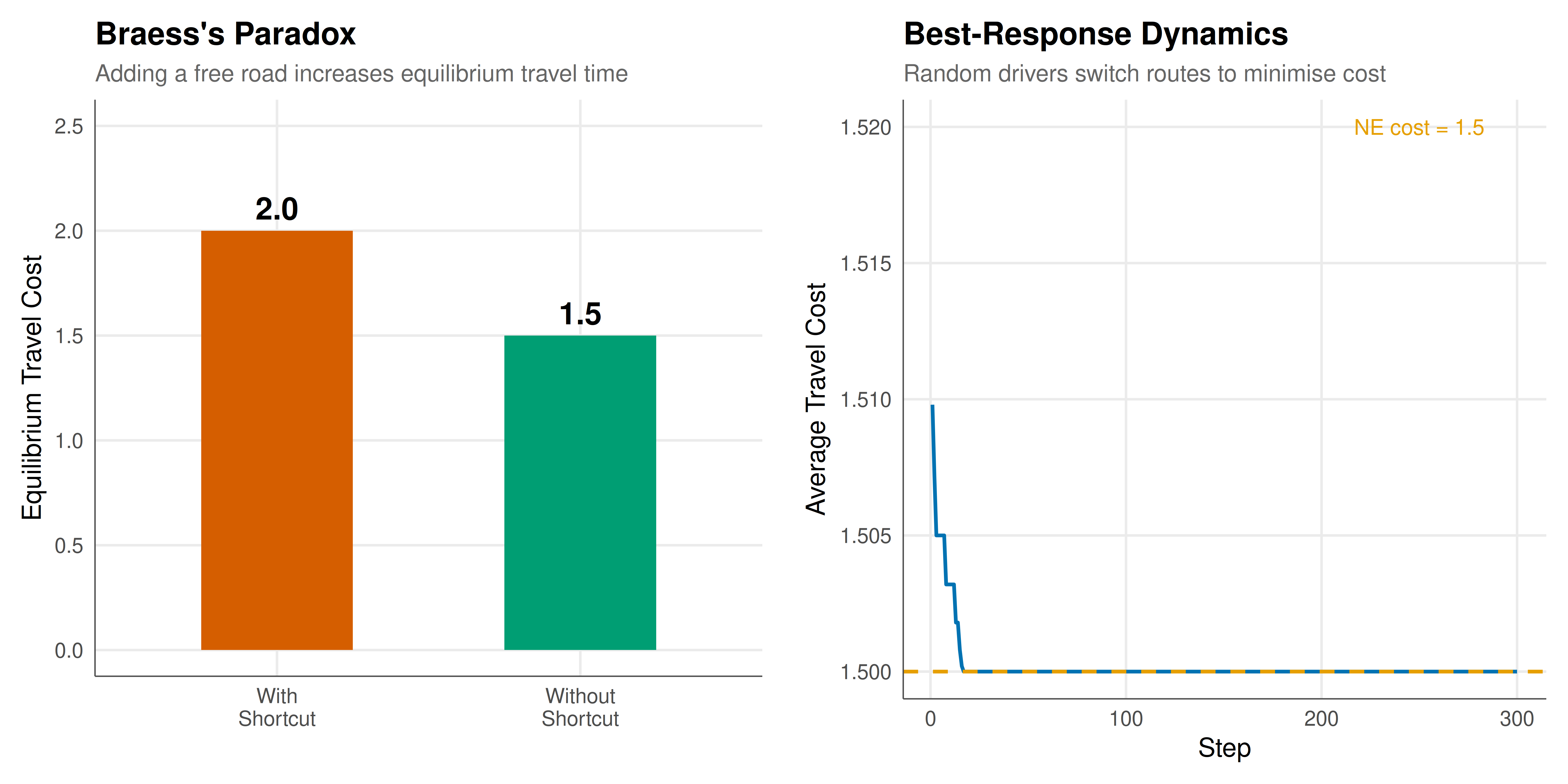
#| fig-cap: "Figure 1. Braess's paradox in a traffic network. Left: equilibrium travel costs with and without the shortcut road -- adding the free shortcut increases cost from 1.5 to 2.0. Right: best-response dynamics showing convergence to the Nash equilibrium."
#| dev: [png, pdf]
#| fig-width: 10
#| fig-height: 5
#| dpi: 300
# Left panel: Braess's paradox comparison
braess_data <- data.frame(
  scenario = c("Without\nShortcut", "With\nShortcut"),
  cost = c(1.5, 2.0),
  fill_col = c("No shortcut", "With shortcut")
)

p_braess <- ggplot(braess_data, aes(x = scenario, y = cost, fill = fill_col)) +
  geom_col(width = 0.5) +
  geom_text(aes(label = sprintf("%.1f", cost)), vjust = -0.5, size = 5,
            fontface = "bold") +
  scale_fill_manual(values = okabe_ito[c(3, 6)], name = "") +
  labs(
    title = "Braess's Paradox",
    subtitle = "Adding a free road increases equilibrium travel time",
    x = "", y = "Equilibrium Travel Cost"
  ) +
  theme_publication() +
  coord_cartesian(ylim = c(0, 2.5)) +
  theme(legend.position = "none")

# Right panel: Best-response dynamics convergence
p_brd <- ggplot(brd_no, aes(x = step, y = avg_cost)) +
  geom_line(color = okabe_ito[5], linewidth = 0.8) +
  geom_hline(yintercept = 1.5, linetype = "dashed", color = okabe_ito[1],
             linewidth = 0.8) +
  annotate("text", x = 250, y = 1.52, label = "NE cost = 1.5",
           color = okabe_ito[1], size = 3.5) +
  labs(
    title = "Best-Response Dynamics",
    subtitle = "Random drivers switch routes to minimise cost",
    x = "Step", y = "Average Travel Cost"
  ) +
  theme_publication()

gridExtra::grid.arrange(p_braess, p_brd, ncol = 2)
```
## Interactive figure
The interactive figure shows the flow allocation across different scenarios, letting readers explore the congestion on each edge by hovering.
```{r}
#| label: fig-braess-interactive
# Show flow breakdown by edge for both scenarios
edge_data <- bind_rows(
  data.frame(
    scenario = "Without Shortcut",
    edge = c("O->A", "A->D", "O->B", "B->D", "A->B"),
    flow = c(50, 50, 50, 50, 0),
    cost = c(0.5, 1.0, 1.0, 0.5, 0)
  ),
  data.frame(
    scenario = "With Shortcut",
    edge = c("O->A", "A->D", "O->B", "B->D", "A->B"),
    flow = c(100, 0, 0, 100, 100),
    cost = c(1.0, 0, 0, 1.0, 0)
  )
) %>%
  mutate(label = sprintf("Edge: %s\nFlow: %d drivers\nEdge cost: %.2f\nScenario: %s",
                         edge, flow, cost, scenario))

p_edge <- ggplot(edge_data,
                 aes(x = edge, y = flow, fill = scenario, text = label)) +
  geom_col(position = position_dodge(width = 0.7), width = 0.6) +
  scale_fill_manual(values = okabe_ito[c(3, 6)], name = "Scenario") +
  labs(
    title = "Edge Flows: Braess's Paradox",
    subtitle = "How the shortcut redirects all traffic",
    x = "Network Edge", y = "Number of Drivers"
  ) +
  theme_publication()

ggplotly(p_edge, tooltip = "text") %>%
  config(displaylogo = FALSE)
```
## Interpretation
The results demonstrate Braess's paradox with stark clarity. In the original network without the shortcut, the equilibrium splits 100 drivers equally between the top and bottom routes, each costing 1.5 units. This is the unique Nash equilibrium because any deviation (moving a driver from one route to the other) would increase the deviator's cost: the route they join becomes more congested while the route they leave becomes less congested, but the symmetric structure means the joining cost exceeds the leaving benefit.
When we add the free shortcut from A to B, the equilibrium shifts dramatically. The shortcut route (O->A->B->D) has cost $n_{OA}/100 + 0 + n_{BD}/100$, which is attractive precisely because it combines the two congestion-sensitive edges. In equilibrium, all 100 drivers use the shortcut, each paying a cost of $100/100 + 0 + 100/100 = 2.0$. This is higher than the original 1.5! No individual driver wants to switch to the top or bottom route because those routes still cost 2.0 as well (since all traffic flows through O->A and B->D). The paradox arises because the shortcut creates a prisoners' dilemma: each driver individually benefits from using it, but collectively they are all worse off.
The best-response dynamics simulation confirms the theoretical prediction: starting from a random allocation, the process converges to the equilibrium as drivers sequentially switch to lower-cost routes. The convergence is guaranteed by Rosenthal's potential function argument, as each improving switch reduces the potential. The convergence speed depends on the initial allocation and the order of switches, but termination is always finite.
Braess's paradox has profound implications for infrastructure planning. It shows that naive capacity expansion (adding roads, network links, or server capacity) can backfire if it changes the equilibrium in an adverse way. The paradox has motivated research into mechanism design for networks (tolling, capacity design) and the concept of the **price of anarchy**, which measures the worst-case ratio between the equilibrium cost and the social optimum.
## Extensions & related tutorials
Congestion games connect to many areas of game theory and network science. The price of anarchy quantifies how much worse selfish routing is compared to socially optimal routing. Mechanism design for networks asks how to set tolls or design capacity to improve equilibrium outcomes. Evolutionary dynamics on networks provide an alternative perspective on how populations converge to equilibria.
- [Diffusion and cascades on networks](../../network-science/diffusion-cascades-networks/)
- [Fictitious play and convergence](../../ml-and-gt/fictitious-play-convergence/)
- [LP duality and zero-sum game solutions](../../linear-algebra-matrix/lp-duality-zero-sum/)
- [Support enumeration algorithm for Nash equilibria](../../optimization-numerical-methods/support-enumeration-algorithm/)
## References
::: {#refs}
:::