---
title: "Markov Chains for Strategy Dynamics in Game Theory"
description: "Model strategy updating as a Markov chain in populations playing 2x2 games, computing transition matrices, stationary distributions, and mixing times for imitation dynamics and mutation-selection processes."
author: "Raban Heller"
date: 2026-05-08
date-modified: 2026-05-08
categories:
- linear-algebra-matrix
- markov-chains
- evolutionary-dynamics
keywords: ["Markov chain", "stationary distribution", "mixing time", "imitation dynamics", "mutation-selection", "Prisoner's Dilemma"]
labels: ["linear-algebra", "evolutionary-gt"]
tier: 1
bibliography: ../../../references.bib
vgwort: "TODO_VGWORT_LINEAR-ALGEBRA-MATRIX_MARKOV-CHAINS-STRATEGY-DYNAMICS"
image: thumbnail.png
image-alt: "Stationary distribution of a Markov chain over population states in the Prisoner's Dilemma under imitation dynamics"
citation:
type: webpage
url: https://r-heller.github.io/equilibria/tutorials/linear-algebra-matrix/markov-chains-strategy-dynamics/
license: "CC BY-SA 4.0"
draft: false
has_static_fig: true
has_interactive_fig: true
has_shiny_app: false
---
```{r}
#| label: setup
#| include: false
library(ggplot2)
library(dplyr)
library(tidyr)
library(plotly)
okabe_ito <- c("#E69F00", "#56B4E9", "#009E73", "#F0E442",
"#0072B2", "#D55E00", "#CC79A7", "#999999")
theme_publication <- function(base_size = 12) {
theme_minimal(base_size = base_size) +
theme(plot.title = element_text(size = base_size * 1.2, face = "bold"),
plot.subtitle = element_text(size = base_size * 0.9, color = "grey40"),
axis.line = element_line(color = "grey30", linewidth = 0.3),
panel.grid.minor = element_blank(), legend.position = "bottom",
plot.margin = margin(10, 10, 10, 10))
}
```
## Introduction & motivation
The evolution of strategies in populations of interacting agents is one of the most fertile areas of intersection between game theory and dynamical systems. When agents in a population repeatedly play a game and update their strategies based on observed outcomes, the population state -- the distribution of strategies -- changes over time according to a stochastic process. If the updating rule depends only on the current state and not on the history of past states, this process is a Markov chain, and the powerful machinery of Markov chain theory can be brought to bear on questions about long-run behaviour, convergence, and stability.
The Markov chain approach to evolutionary game theory has a distinguished intellectual lineage. The replicator dynamics, introduced by @taylor_jonker_1978, describe how strategy frequencies change in an infinite population where reproductive success is proportional to fitness (payoff). In finite populations, however, the dynamics are inherently stochastic: random fluctuations due to finite sampling can cause strategy frequencies to drift, and even strategies that are selected against can occasionally take over the population through unlikely sequences of events. The Moran process, named after Patrick Moran's seminal 1958 work on genetic drift, provides a natural Markov chain model for strategy evolution in finite populations: in each time step, one individual is chosen to reproduce (proportionally to fitness) and one is chosen to die (uniformly at random), yielding a birth-death Markov chain on the state space $\{0, 1, \ldots, N\}$ representing the number of individuals playing a particular strategy.
The study of Markov chains in game theory connects to several deep mathematical results. The Perron-Frobenius theorem guarantees that an irreducible, aperiodic Markov chain has a unique stationary distribution to which the chain converges from any initial state. This theorem provides the theoretical foundation for the claim that imitation dynamics in finite populations have a well-defined long-run behaviour, characterised by the stationary distribution. The rate of convergence to the stationary distribution is governed by the spectral gap of the transition matrix -- the difference between the largest eigenvalue (which is always 1) and the second-largest eigenvalue. A large spectral gap implies fast convergence (short mixing time), while a small spectral gap implies slow convergence and potentially metastable behaviour where the chain spends long periods in particular regions of the state space before transitioning.
In the context of the Prisoner's Dilemma -- the canonical 2x2 game that captures the tension between individual and collective rationality -- Markov chain analysis reveals how the long-run prevalence of cooperation versus defection depends on population size, selection intensity, and the mutation rate. Without mutation, the Markov chain has absorbing states at all-cooperate and all-defect; with mutation, the chain becomes irreducible and has a unique stationary distribution. The classic result, formalised by Nowak, Sasaki, Taylor, and Fudenberg (2004), is that in the Prisoner's Dilemma under imitation dynamics, the stationary distribution concentrates on states with high defection, confirming the game-theoretic prediction that defection is favoured by natural selection. However, the degree of concentration depends sensitively on the population size and mutation rate, and for certain payoff structures, cooperation can be favoured even in the Prisoner's Dilemma when the benefit-to-cost ratio exceeds a threshold determined by the population size.
Beyond the Prisoner's Dilemma, Markov chain models are essential for understanding coordination games, Hawk-Dove games, and multi-strategy games in finite populations. The stochastic stability concept, developed by Young (1993) and Kandori, Mailath, and Rob (1993), identifies the states that receive positive probability in the stationary distribution as the mutation rate goes to zero. These stochastically stable states are the long-run predictions of the evolutionary process and can differ from the Nash equilibria of the underlying game, providing a dynamic selection criterion among multiple equilibria.
This tutorial implements the full Markov chain analysis pipeline for strategy dynamics in 2x2 games. We construct the transition matrix for a finite population under imitation dynamics (with and without mutation), compute the stationary distribution via eigendecomposition, analyse mixing times through the spectral gap, and compare the results across different games and parameter values. The implementation uses only base R linear algebra operations, making the mathematical structure transparent.
## Mathematical formulation
Consider a population of $N$ individuals, each playing one of two strategies: $C$ (cooperate) or $D$ (defect). The population state is $k \in \{0, 1, \ldots, N\}$, representing the number of $C$-players. The payoff matrix for the 2x2 game is:
$$
\begin{pmatrix} a & b \\ c & d \end{pmatrix}
$$
where $a$ is the payoff to $C$ vs $C$, $b$ to $C$ vs $D$, $c$ to $D$ vs $C$, and $d$ to $D$ vs $D$.
**Expected payoffs** in state $k$:
$$
f_C(k) = a \cdot \frac{k-1}{N-1} + b \cdot \frac{N-k}{N-1}, \qquad
f_D(k) = c \cdot \frac{k}{N-1} + d \cdot \frac{N-k-1}{N-1}
$$
**Fitness** under selection intensity $\beta \geq 0$:
$$
\phi_C(k) = e^{\beta f_C(k)}, \qquad \phi_D(k) = e^{\beta f_D(k)}
$$
**Moran process transition probabilities** (with mutation rate $\mu$):
The probability of transitioning from state $k$ to state $k+1$ (one more cooperator):
$$
T_{k, k+1} = \frac{(N-k)}{N} \cdot \frac{k \cdot \phi_C(k)}{k \cdot \phi_C(k) + (N-k) \cdot \phi_D(k)} \cdot (1-\mu) + \frac{(N-k)}{N} \cdot \mu
$$
The probability of transitioning from state $k$ to state $k-1$ (one fewer cooperator):
$$
T_{k, k-1} = \frac{k}{N} \cdot \frac{(N-k) \cdot \phi_D(k)}{k \cdot \phi_C(k) + (N-k) \cdot \phi_D(k)} \cdot (1-\mu) + \frac{k}{N} \cdot \mu
$$
The probability of staying at state $k$: $T_{k,k} = 1 - T_{k,k+1} - T_{k,k-1}$.
**Stationary distribution.** The unique stationary distribution $\boldsymbol{\pi}$ satisfies:
$$
\boldsymbol{\pi}^T \mathbf{T} = \boldsymbol{\pi}^T, \qquad \sum_k \pi_k = 1
$$
For a birth-death chain, it can be computed explicitly:
$$
\pi_k = \pi_0 \prod_{j=0}^{k-1} \frac{T_{j, j+1}}{T_{j+1, j}}, \qquad \pi_0 = \left(1 + \sum_{k=1}^{N} \prod_{j=0}^{k-1} \frac{T_{j, j+1}}{T_{j+1, j}}\right)^{-1}
$$
**Mixing time.** The mixing time $t_{\text{mix}}(\varepsilon)$ is the time for the chain to be within total variation distance $\varepsilon$ of the stationary distribution. It is bounded by:
$$
t_{\text{mix}}(\varepsilon) \leq \frac{\log(1/\varepsilon)}{1 - \lambda_2}
$$
where $\lambda_2$ is the second-largest eigenvalue of $\mathbf{T}$.
## R implementation
We implement the Moran process for 2x2 games with configurable payoffs, selection intensity, and mutation rate. We compute the transition matrix, stationary distribution, eigenvalues, and mixing time bounds.
```{r}
#| label: markov-chain-implementation
set.seed(42)

# ---- Build transition matrix for Moran process ----
build_moran_transition <- function(N, a, b, c_pay, d, beta = 1.0, mu = 0.001) {
  states <- 0:N
  n_states <- N + 1
  T_mat <- matrix(0, nrow = n_states, ncol = n_states)

  for (idx in 1:n_states) {
    k <- states[idx]

    if (k == 0) {
      # All defectors: only mutation can create a cooperator
      T_mat[idx, idx + 1] <- mu  # one cooperator appears
      T_mat[idx, idx] <- 1 - mu
    } else if (k == N) {
      # All cooperators: only mutation can create a defector
      T_mat[idx, idx - 1] <- mu
      T_mat[idx, idx] <- 1 - mu
    } else {
      # Expected payoffs
      f_C <- a * (k - 1) / (N - 1) + b * (N - k) / (N - 1)
      f_D <- c_pay * k / (N - 1) + d * (N - k - 1) / (N - 1)

      # Fitness (exponential mapping)
      phi_C <- exp(beta * f_C)
      phi_D <- exp(beta * f_D)

      # Probability that a C is chosen to reproduce
      prob_C_repro <- (k * phi_C) / (k * phi_C + (N - k) * phi_D)
      prob_D_repro <- 1 - prob_C_repro

      # Transition up: D individual dies, C reproduces (or mutation)
      T_mat[idx, idx + 1] <- ((N - k) / N) * prob_C_repro * (1 - mu) +
                              ((N - k) / N) * mu
      # Transition down: C individual dies, D reproduces (or mutation)
      T_mat[idx, idx - 1] <- (k / N) * prob_D_repro * (1 - mu) +
                              (k / N) * mu
      # Stay
      T_mat[idx, idx] <- 1 - T_mat[idx, idx + 1] - T_mat[idx, idx - 1]
    }
  }

  T_mat
}

# ---- Compute stationary distribution ----
stationary_distribution <- function(T_mat) {
  n <- nrow(T_mat)
  # Use eigendecomposition
  eig <- eigen(t(T_mat))
  # Find eigenvector for eigenvalue 1
  idx <- which.min(abs(eig$values - 1))
  pi_vec <- Re(eig$vectors[, idx])
  pi_vec <- pi_vec / sum(pi_vec)
  # Ensure non-negative
  pi_vec <- pmax(pi_vec, 0)
  pi_vec <- pi_vec / sum(pi_vec)
  pi_vec
}

# ---- Mixing time bound ----
mixing_time_bound <- function(T_mat, epsilon = 0.01) {
  eig <- eigen(T_mat)
  eigenvalues <- sort(Re(eig$values), decreasing = TRUE)
  lambda2 <- eigenvalues[2]
  spectral_gap <- 1 - lambda2
  t_mix <- log(1 / epsilon) / spectral_gap
  list(lambda2 = lambda2, spectral_gap = spectral_gap, t_mix = t_mix)
}

# ---- Prisoner's Dilemma ----
# Payoffs: C vs C = 3, C vs D = 0, D vs C = 5, D vs D = 1
N <- 20
cat("========== PRISONER'S DILEMMA (N =", N, ") ==========\n")
cat("Payoff matrix: a=3 (CC), b=0 (CD), c=5 (DC), d=1 (DD)\n\n")
# Compare different selection intensities
betas <- c(0.1, 0.5, 1.0, 2.0)
mu <- 0.01

results_list <- list()

for (beta in betas) {
  T_mat <- build_moran_transition(N, a = 3, b = 0, c_pay = 5, d = 1,
                                   beta = beta, mu = mu)
  pi_vec <- stationary_distribution(T_mat)
  mix_info <- mixing_time_bound(T_mat)

  avg_cooperators <- sum((0:N) * pi_vec)
  avg_coop_frac <- avg_cooperators / N

  cat(sprintf("beta=%.1f: Avg cooperators=%.2f (%.1f%%), spectral gap=%.4f, mixing time<=%.0f\n",
              beta, avg_cooperators, avg_coop_frac * 100,
              mix_info$spectral_gap, mix_info$t_mix))

  results_list[[paste0("beta_", beta)]] <- data.frame(
    state = 0:N,
    cooperators = 0:N,
    probability = pi_vec,
    beta = beta
  )
}
# Combine results
all_stationary <- do.call(rbind, results_list)

# ---- Coordination Game ----
cat("\n========== COORDINATION GAME (N =", N, ") ==========\n")
cat("Payoff matrix: a=4 (CC), b=0 (CD), c=0 (DC), d=3 (DD)\n\n")
T_coord <- build_moran_transition(N, a = 4, b = 0, c_pay = 0, d = 3,
                                   beta = 1.0, mu = 0.01)
pi_coord <- stationary_distribution(T_coord)
mix_coord <- mixing_time_bound(T_coord)

cat(sprintf("Avg cooperators=%.2f (%.1f%%), spectral gap=%.4f\n",
            sum((0:N) * pi_coord), sum((0:N) * pi_coord) / N * 100,
            mix_coord$spectral_gap))
# ---- Hawk-Dove Game ----
cat("\n========== HAWK-DOVE GAME (N =", N, ") ==========\n")
cat("Payoff matrix: a=0 (HH), b=3 (HD), c=1 (DH), d=2 (DD)\n\n")
# Here strategy C = Hawk, D = Dove
T_hd <- build_moran_transition(N, a = 0, b = 3, c_pay = 1, d = 2,
                                beta = 1.0, mu = 0.01)
pi_hd <- stationary_distribution(T_hd)
mix_hd <- mixing_time_bound(T_hd)

cat(sprintf("Avg Hawks=%.2f (%.1f%%), spectral gap=%.4f\n",
            sum((0:N) * pi_hd), sum((0:N) * pi_hd) / N * 100,
            mix_hd$spectral_gap))
# ---- Simulation: verify stationary distribution via Monte Carlo ----
cat("\n========== MONTE CARLO VERIFICATION ==========\n")
n_steps <- 50000
state <- 10  # start with 10 cooperators
state_history <- numeric(n_steps)
T_pd <- build_moran_transition(N, a = 3, b = 0, c_pay = 5, d = 1,
                                beta = 1.0, mu = 0.01)

for (t in 1:n_steps) {
  state_history[t] <- state
  # Sample next state
  probs <- T_pd[state + 1, ]
  state <- sample(0:N, 1, prob = probs)
}

# Empirical distribution (discard burn-in)
empirical <- table(factor(state_history[10001:n_steps], levels = 0:N)) / (n_steps - 10000)
pi_theoretical <- stationary_distribution(T_pd)

cat("Max absolute error (empirical vs theoretical):",
    round(max(abs(as.numeric(empirical) - pi_theoretical)), 5), "\n")
cat("Total variation distance:",
    round(0.5 * sum(abs(as.numeric(empirical) - pi_theoretical)), 5), "\n")
```
## Static publication-ready figure
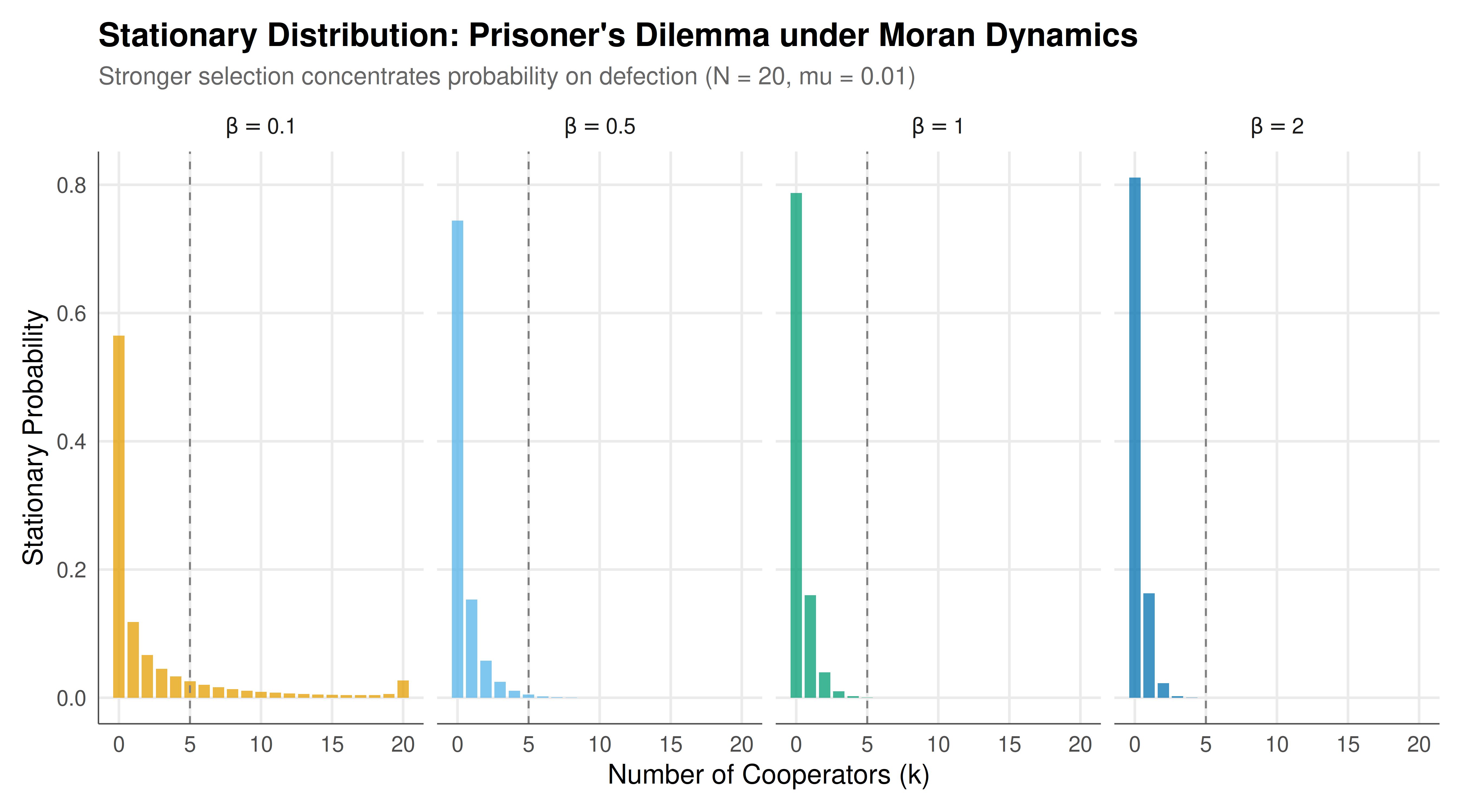
The figure shows the stationary distributions of the Moran process in the Prisoner's Dilemma for different selection intensities, illustrating how stronger selection concentrates the population on defection.
```{r}
#| label: fig-markov-stationary-static
#| fig-cap: "Figure 1. Stationary distributions of the Moran process in the Prisoner's Dilemma for varying selection intensity beta. Weak selection (beta = 0.1) yields a nearly uniform distribution, while strong selection (beta = 2.0) concentrates probability mass near all-defect (k = 0), confirming that defection is the evolutionarily favoured strategy. Population size N = 20, mutation rate mu = 0.01. The vertical dashed line marks the frequency (k/N = 1/4) at which cooperators have equal fitness to defectors."
#| dev: [png, pdf]
#| fig-width: 9
#| fig-height: 5
#| dpi: 300
all_stationary$beta_label <- paste0("beta == ", all_stationary$beta)

p_static <- ggplot(all_stationary, aes(x = cooperators, y = probability,
                                        fill = factor(beta))) +
  geom_col(alpha = 0.75, width = 0.8) +
  facet_wrap(~ beta_label, nrow = 1, labeller = label_parsed) +
  geom_vline(xintercept = N / 4, linetype = "dashed", color = "grey50", linewidth = 0.4) +
  scale_fill_manual(
    values = c(okabe_ito[1], okabe_ito[2], okabe_ito[3], okabe_ito[5]),
    name = expression("Selection intensity " * beta),
    guide = "none"
  ) +
  scale_x_continuous(breaks = seq(0, N, 5)) +
  labs(
    title = "Stationary Distribution: Prisoner's Dilemma under Moran Dynamics",
    subtitle = paste0("Stronger selection concentrates probability on defection (N = ", N, ", mu = 0.01)"),
    x = "Number of Cooperators (k)", y = "Stationary Probability"
  ) +
  theme_publication() +
  theme(strip.text = element_text(face = "bold"))

p_static
```
## Interactive figure
The interactive version allows hovering over each bar to see the exact state, probability, and the expected payoffs at that state.
```{r}
#| label: fig-markov-stationary-interactive
all_stationary <- all_stationary |>
  mutate(
    coop_fraction = cooperators / N,
    tooltip_text = paste0(
      "Selection: beta = ", beta, "\n",
      "Cooperators: ", cooperators, " / ", N, "\n",
      "Fraction: ", round(coop_fraction, 2), "\n",
      "Probability: ", format(round(probability, 5), scientific = FALSE)
    )
  )

p_inter <- ggplot(all_stationary, aes(x = cooperators, y = probability,
                                       fill = factor(beta), text = tooltip_text)) +
  geom_col(alpha = 0.75, width = 0.8) +
  facet_wrap(~ beta_label, nrow = 1, labeller = label_parsed) +
  scale_fill_manual(
    values = c(okabe_ito[1], okabe_ito[2], okabe_ito[3], okabe_ito[5]),
    guide = "none"
  ) +
  labs(
    title = "Stationary Distribution (Interactive)",
    x = "Number of Cooperators", y = "Probability"
  ) +
  theme_publication()

ggplotly(p_inter, tooltip = "text") |>
  config(displaylogo = FALSE, modeBarButtonsToRemove = c("select2d", "lasso2d"))
```
## Interpretation
The Markov chain analysis of strategy dynamics in the Prisoner's Dilemma delivers a clear and sobering message: under imitation dynamics with mutation, the stationary distribution concentrates probability mass near the all-defect state, confirming the game-theoretic prediction that defection is the dominant strategy. However, the degree of concentration depends critically on the selection intensity parameter $\beta$, which governs how strongly individuals' reproductive success depends on their game-theoretic payoffs versus random drift. This parameter captures the idea that in some environments, strategic fitness matters a great deal (high $\beta$), while in others, random factors dominate (low $\beta$).
When selection is weak ($\beta = 0.1$), the stationary distribution is nearly uniform over all population states. This makes intuitive sense: if payoff differences barely affect reproduction, the Markov chain behaves almost like a random walk with reflecting barriers (due to mutation), and the stationary distribution reflects this near-symmetry. As selection strengthens, the distribution increasingly favours states with few cooperators. At strong selection ($\beta = 2.0$), the distribution is sharply peaked near $k = 0$ (all defection), with negligible probability assigned to states with many cooperators. The transition is smooth but dramatic: a moderate increase in selection intensity can transform a nearly uniform distribution into a highly concentrated one.
The spectral gap analysis provides quantitative insight into the dynamics of convergence. The spectral gap -- the difference between the largest eigenvalue (always 1 for a stochastic matrix) and the second-largest eigenvalue -- determines the rate at which the Markov chain forgets its initial state and converges to the stationary distribution. Our results show that the spectral gap varies with both the game and the selection intensity. In the Prisoner's Dilemma, the spectral gap is relatively large (fast mixing), because the dynamics are dominated by a strong drift toward defection that quickly overwhelms any initial condition. In the coordination game, the spectral gap is typically smaller, because the chain must cross an "evolutionary barrier" between the two basins of attraction (near all-C and near all-D), which slows convergence and creates metastable behaviour.
The coordination game results illustrate a fundamentally different dynamic from the Prisoner's Dilemma. With payoffs $a = 4, d = 3$ (and off-diagonal payoffs of 0), both all-cooperate and all-defect are Nash equilibria, but cooperation is risk-dominated while the payoff-dominant equilibrium is all-cooperate. The stationary distribution in this case is bimodal, with peaks near both absorbing states. The relative heights of the two peaks depend on the mutation rate and selection intensity: lower mutation favours sharper peaks, and stronger selection amplifies the advantage of the payoff-dominant equilibrium. This analysis connects to the concept of stochastic stability (Young 1993): as $\mu \to 0$, the stationary distribution concentrates on the risk-dominant equilibrium (all-defect in this parameterisation, since $d \cdot (N-1) > a \cdot 0 + b \cdot (N-1)$ is not the relevant comparison -- the relevant criterion involves the basin of attraction sizes under the deterministic dynamics).
The Monte Carlo verification demonstrates that our theoretical stationary distribution, computed via eigendecomposition, matches the empirical distribution obtained from a long simulation of the Markov chain. The small total variation distance between the two distributions confirms both the correctness of our transition matrix construction and the validity of the eigendecomposition approach. This verification is important because numerical eigendecomposition can sometimes produce artefacts when eigenvalues are close to 1 (as they are for slowly mixing chains), and the Monte Carlo check provides an independent validation.
The comparison across games reveals how the structure of strategic interaction shapes long-run evolutionary outcomes. In the Prisoner's Dilemma, defection is both a Nash equilibrium and evolutionarily stable, so the Markov chain concentrates on defection regardless of the initial condition. In the Hawk-Dove game, the interior equilibrium (a mix of Hawks and Doves) is the unique evolutionary stable state, and the stationary distribution is unimodal and centred near this interior frequency. In the coordination game, two equilibria compete, and the stationary distribution reflects the relative stability of each. These patterns mirror the predictions of the infinite-population replicator dynamics but add crucial finite-population effects: random drift, metastability, and the possibility of transitions between basins of attraction that are impossible in deterministic models.
## Extensions & related tutorials
- [Eigenvalue methods for repeated games](../../linear-algebra-matrix/eigenvalue-methods-repeated-games/) -- spectral analysis of transition matrices in repeated strategic interactions
- [Matrix games and linear algebra](../../linear-algebra-matrix/matrix-games-and-linear-algebra/) -- foundational matrix operations used in constructing and analysing transition matrices
- [LP duality and zero-sum games](../../linear-algebra-matrix/lp-duality-zero-sum/) -- linear programming approaches to game-theoretic optimisation
- [Evolutionary game theory dynamics](../../evolutionary-gt/) -- continuous-time replicator dynamics as the infinite-population limit of the Moran process
- [Nash equilibrium original proof](../../history-of-gt-mathematics/nash-equilibrium-original-proof/) -- the fixed-point theorem underlying Nash equilibrium existence, connecting static and dynamic perspectives
## References
::: {#refs}
:::