---
title: "Eigenvalue methods for repeated game analysis"
description: "Use eigenvalue decomposition to compute stationary distributions, convergence rates, and long-run cooperation levels for Markov strategies in the repeated Prisoner's Dilemma, including Tit-for-Tat, Grim Trigger, and stochastic strategies."
author: "Raban Heller"
date: 2026-05-08
date-modified: 2026-05-08
categories:
- linear-algebra-matrix
- repeated-games
- markov-chains
- eigenvalue-decomposition
keywords: ["eigenvalue decomposition", "Markov chain", "stationary distribution", "spectral gap", "Tit-for-Tat", "repeated Prisoner's Dilemma", "convergence rate", "stochastic strategies", "cooperation"]
labels: ["linear-algebra-matrix", "repeated-games"]
tier: 1
bibliography: ../../../references.bib
vgwort: "TODO_VGWORT_linear-algebra-matrix_eigenvalue-methods-repeated-games"
image: thumbnail.png
image-alt: "Eigenvalue spectrum plot showing the dominant eigenvalue at 1 and subdominant eigenvalues determining convergence rate for different strategy matchups in the repeated Prisoner's Dilemma"
citation:
type: webpage
url: https://r-heller.github.io/equilibria/tutorials/linear-algebra-matrix/eigenvalue-methods-repeated-games/
license: "CC BY-SA 4.0"
draft: false
has_static_fig: true
has_interactive_fig: true
has_shiny_app: false
---
```{r}
#| label: setup
#| include: false
library(ggplot2)
library(dplyr)
library(tidyr)
library(plotly)
okabe_ito <- c("#E69F00", "#56B4E9", "#009E73", "#F0E442",
"#0072B2", "#D55E00", "#CC79A7", "#999999")
theme_publication <- function(base_size = 12) {
theme_minimal(base_size = base_size) +
theme(plot.title = element_text(size = base_size * 1.2, face = "bold"),
plot.subtitle = element_text(size = base_size * 0.9, color = "grey40"),
axis.line = element_line(color = "grey30", linewidth = 0.3),
panel.grid.minor = element_blank(), legend.position = "bottom",
plot.margin = margin(10, 10, 10, 10))
}
```
## Introduction & motivation
The repeated Prisoner's Dilemma (RPD) is the canonical model for studying how cooperation can emerge and persist among self-interested agents. Robert Axelrod's celebrated tournaments showed that Tit-for-Tat --- the strategy that cooperates initially and then mirrors the opponent's previous move --- performs remarkably well against a diverse population of strategies [@axelrod_1984]. But *why* does Tit-for-Tat succeed, and how quickly do different strategy matchups converge to their long-run behaviour?
The answer lies in eigenvalue decomposition. When two players in a repeated game use Markov strategies --- strategies that condition only on the current state of play, not the entire history --- the sequence of states forms a finite Markov chain. The transition matrix of this chain encodes everything about the long-run dynamics: the stationary distribution tells us the long-run frequency of each outcome (mutual cooperation, mutual defection, or the two asymmetric outcomes), and the eigenvalue spectrum determines how fast the chain converges to this stationary distribution.
Specifically, every stochastic transition matrix $M$ has a dominant eigenvalue $\lambda_1 = 1$ (corresponding to the stationary distribution), and the rate of convergence is governed by the **spectral gap** $1 - |\lambda_2|$, where $\lambda_2$ is the second-largest eigenvalue in absolute value. A large spectral gap means rapid convergence to the long-run frequencies; a small spectral gap means the chain "remembers" its initial state for a long time. This has direct game-theoretic implications: if convergence is slow, the early rounds of the game matter more, and the initial state (who cooperated or defected first) has a lasting influence on average payoffs.
In this tutorial, we construct the transition matrices for several classic strategy matchups in the repeated Prisoner's Dilemma, compute their eigenvalue decompositions, derive stationary distributions and spectral gaps, and visualise how these mathematical quantities translate into long-run cooperation levels and convergence dynamics. The approach generalises beyond the Prisoner's Dilemma to any repeated game where players use Markov (or "memory-one") strategies, including models of animal conflict, firm competition, and international relations.
The mathematical framework we develop connects three seemingly separate concepts: (1) the strategy pair chosen by the players, (2) the algebraic properties of the resulting transition matrix, and (3) the observable dynamics of cooperation and defection over time. By making these connections explicit through eigenvalue decomposition, we obtain a unified analytical tool for understanding the dynamics of any Markov strategy interaction.
## Mathematical formulation
**Markov strategies in the RPD.** The Prisoner's Dilemma has four possible stage-game outcomes, which we label as states: $CC$ (both cooperate), $CD$ (Player 1 cooperates, Player 2 defects), $DC$ (Player 1 defects, Player 2 cooperates), and $DD$ (both defect). A memory-one (Markov) strategy for Player 1 is a vector $\mathbf{p} = (p_{CC}, p_{CD}, p_{DC}, p_{DD})$, where $p_s$ is the probability that Player 1 cooperates in the next round given that the current state is $s$. Similarly, Player 2's strategy is $\mathbf{q} = (q_{CC}, q_{CD}, q_{DC}, q_{DD})$.
**Transition matrix.** Given strategies $\mathbf{p}$ and $\mathbf{q}$, the $4 \times 4$ transition matrix $M$ has entries:
$$
M_{CC \to CC} = p_{CC} \cdot q_{CC}, \quad M_{CC \to CD} = p_{CC} \cdot (1 - q_{CC})
$$
$$
M_{CC \to DC} = (1 - p_{CC}) \cdot q_{CC}, \quad M_{CC \to DD} = (1 - p_{CC}) \cdot (1 - q_{CC})
$$
and similarly for rows $CD$, $DC$, and $DD$. Each row sums to 1.
**Stationary distribution.** The stationary distribution $\boldsymbol{\pi}$ satisfies $\boldsymbol{\pi}^\top M = \boldsymbol{\pi}^\top$, i.e., $\boldsymbol{\pi}$ is the left eigenvector of $M$ corresponding to eigenvalue $\lambda_1 = 1$, normalised to sum to 1. The long-run cooperation rate for Player 1 is $\pi_{CC} + \pi_{CD}$.
**Spectral gap and convergence.** Let $\lambda_1 = 1 \geq |\lambda_2| \geq |\lambda_3| \geq |\lambda_4|$ be the eigenvalues of $M$ sorted by absolute value. The **spectral gap** is:
$$
\gamma = 1 - |\lambda_2|
$$
The distance between the state distribution at time $t$ and the stationary distribution decays as:
$$
\| \mathbf{v}^{(t)} - \boldsymbol{\pi} \| \leq C \cdot |\lambda_2|^t
$$
The **mixing time** (number of rounds to get within $\epsilon$ of stationarity) scales as:
$$
t_{\text{mix}}(\epsilon) \sim \frac{\log(1/\epsilon)}{\gamma}
$$
## R implementation
We define several classic Markov strategies, build their transition matrices, compute eigenvalue decompositions, and analyse convergence dynamics.
```{r}
#| label: eigenvalue-computation
# --- Define Markov strategies ---
# Format: (p_CC, p_CD, p_DC, p_DD)
strategies <- list(
  "Tit-for-Tat"    = c(1, 0, 1, 0),     # Mirror opponent's last move
  "Grim Trigger"   = c(1, 0, 0, 0),     # Cooperate until first defection, then defect forever
  "Always Cooperate" = c(1, 1, 1, 1),
  "Always Defect"  = c(0, 0, 0, 0),
  "Generous TFT"   = c(1, 0.1, 1, 0.1), # TFT with 10% forgiveness
  "Suspicious TFT" = c(1, 0, 1, 0),     # Same as TFT but defects first (handled via initial state)
  "Pavlov"         = c(1, 0, 0, 1),     # Win-stay, lose-shift
  "Random (50-50)" = c(0.5, 0.5, 0.5, 0.5)
)

# --- Build transition matrix ---
build_transition_matrix <- function(p, q) {
  # States: CC, CD, DC, DD
  # p = (p_CC, p_CD, p_DC, p_DD) for Player 1
  # q = (q_CC, q_CD, q_DC, q_DD) for Player 2
  states <- c("CC", "CD", "DC", "DD")
  M <- matrix(0, 4, 4, dimnames = list(states, states))

  for (s in 1:4) {
    p_coop <- p[s]  # Prob P1 cooperates given state s
    q_coop <- q[s]  # Prob P2 cooperates given state s
    M[s, 1] <- p_coop * q_coop           # -> CC
    M[s, 2] <- p_coop * (1 - q_coop)     # -> CD
    M[s, 3] <- (1 - p_coop) * q_coop     # -> DC
    M[s, 4] <- (1 - p_coop) * (1 - q_coop) # -> DD
  }
  M
}

# --- Eigenvalue analysis ---
analyse_markov <- function(M) {
  eig <- eigen(t(M))  # Left eigenvectors are right eigenvectors of M^T
  # Find eigenvalue closest to 1
  idx1 <- which.min(abs(eig$values - 1))
  stationary <- Re(eig$vectors[, idx1])
  stationary <- stationary / sum(stationary)

  eigenvalues <- eig$values
  # Sort by absolute value (descending)
  ord <- order(Mod(eigenvalues), decreasing = TRUE)
  eigenvalues <- eigenvalues[ord]

  spectral_gap <- 1 - Mod(eigenvalues[2])
  mixing_time <- if (spectral_gap > 1e-10) log(100) / spectral_gap else Inf

  list(
    stationary = stationary,
    eigenvalues = eigenvalues,
    spectral_gap = spectral_gap,
    mixing_time = mixing_time,
    coop_rate_p1 = stationary[1] + stationary[2],
    coop_rate_p2 = stationary[1] + stationary[3]
  )
}

# --- Prisoner's Dilemma payoffs ---
# R=3 (CC), S=0 (CD), T=5 (DC), P=1 (DD)
pd_payoffs <- c(CC = 3, CD = 0, DC = 5, DD = 1)

compute_long_run_payoff <- function(stationary, payoffs = pd_payoffs) {
  sum(stationary * payoffs)
}

# --- Analyse key matchups ---
matchups <- list(
  c("Tit-for-Tat", "Tit-for-Tat"),
  c("Tit-for-Tat", "Always Defect"),
  c("Tit-for-Tat", "Grim Trigger"),
  c("Generous TFT", "Generous TFT"),
  c("Pavlov", "Pavlov"),
  c("Pavlov", "Always Defect"),
  c("Random (50-50)", "Random (50-50)"),
  c("Generous TFT", "Always Defect")
)

results <- list()
for (mu in matchups) {
  p <- strategies[[mu[1]]]
  q <- strategies[[mu[2]]]
  # For P2, swap CD and DC perspectives
  q_adj <- q[c(1, 3, 2, 4)]  # q_CC stays, but CD<->DC swap
  M <- build_transition_matrix(p, q_adj)
  analysis <- analyse_markov(M)

  # Handle degenerate TFT vs TFT case (absorbing states)
  matchup_name <- paste(mu[1], "vs", mu[2])
  payoff_p1 <- compute_long_run_payoff(analysis$stationary)

  results[[matchup_name]] <- list(
    name = matchup_name,
    matrix = M,
    analysis = analysis,
    payoff_p1 = payoff_p1
  )
}

cat("=== Eigenvalue Analysis of Strategy Matchups ===\n\n")
eigen_summary <- tibble(
  matchup = character(),
  lambda_1 = numeric(),
  lambda_2 = numeric(),
  spectral_gap = numeric(),
  mixing_time = numeric(),
  coop_rate = numeric(),
  payoff_p1 = numeric()
)

for (name in names(results)) {
  r <- results[[name]]
  a <- r$analysis
  eigen_summary <- bind_rows(eigen_summary, tibble(
    matchup = name,
    lambda_1 = round(Re(a$eigenvalues[1]), 4),
    lambda_2 = round(Mod(a$eigenvalues[2]), 4),
    spectral_gap = round(a$spectral_gap, 4),
    mixing_time = round(a$mixing_time, 1),
    coop_rate = round(a$coop_rate_p1, 4),
    payoff_p1 = round(r$payoff_p1, 3)
  ))
  cat(sprintf("%-35s | lam2=%.4f | gap=%.4f | t_mix=%.1f | coop=%.3f | payoff=%.3f\n",
              name,
              Mod(a$eigenvalues[2]), a$spectral_gap, a$mixing_time,
              a$coop_rate_p1, r$payoff_p1))
}
# --- Convergence dynamics ---
simulate_convergence <- function(M, initial_state = 1, n_steps = 50) {
  v <- rep(0, 4)
  v[initial_state] <- 1
  states <- c("CC", "CD", "DC", "DD")

  history <- matrix(0, n_steps + 1, 4)
  history[1, ] <- v

  for (t in 1:n_steps) {
    v <- v %*% M
    history[t + 1, ] <- v
  }

  as.data.frame(history) %>%
    setNames(states) %>%
    mutate(time = 0:n_steps) %>%
    pivot_longer(cols = all_of(states), names_to = "state", values_to = "probability")
}

# Simulate convergence for select matchups
conv_data <- list()
for (name in c("Generous TFT vs Generous TFT",
               "Pavlov vs Always Defect",
               "Random (50-50) vs Random (50-50)")) {
  M <- results[[name]]$matrix
  sim <- simulate_convergence(M, initial_state = 4, n_steps = 40) %>%
    mutate(matchup = name)
  conv_data[[name]] <- sim
}

conv_all <- bind_rows(conv_data)

cat("\n=== Stationary Distributions ===\n")
for (name in names(results)) {
  r <- results[[name]]
  cat(sprintf("\n%s:\n", name))
  cat(sprintf("  pi = (CC=%.4f, CD=%.4f, DC=%.4f, DD=%.4f)\n",
              r$analysis$stationary[1], r$analysis$stationary[2],
              r$analysis$stationary[3], r$analysis$stationary[4]))
}
```
## Static publication-ready figure
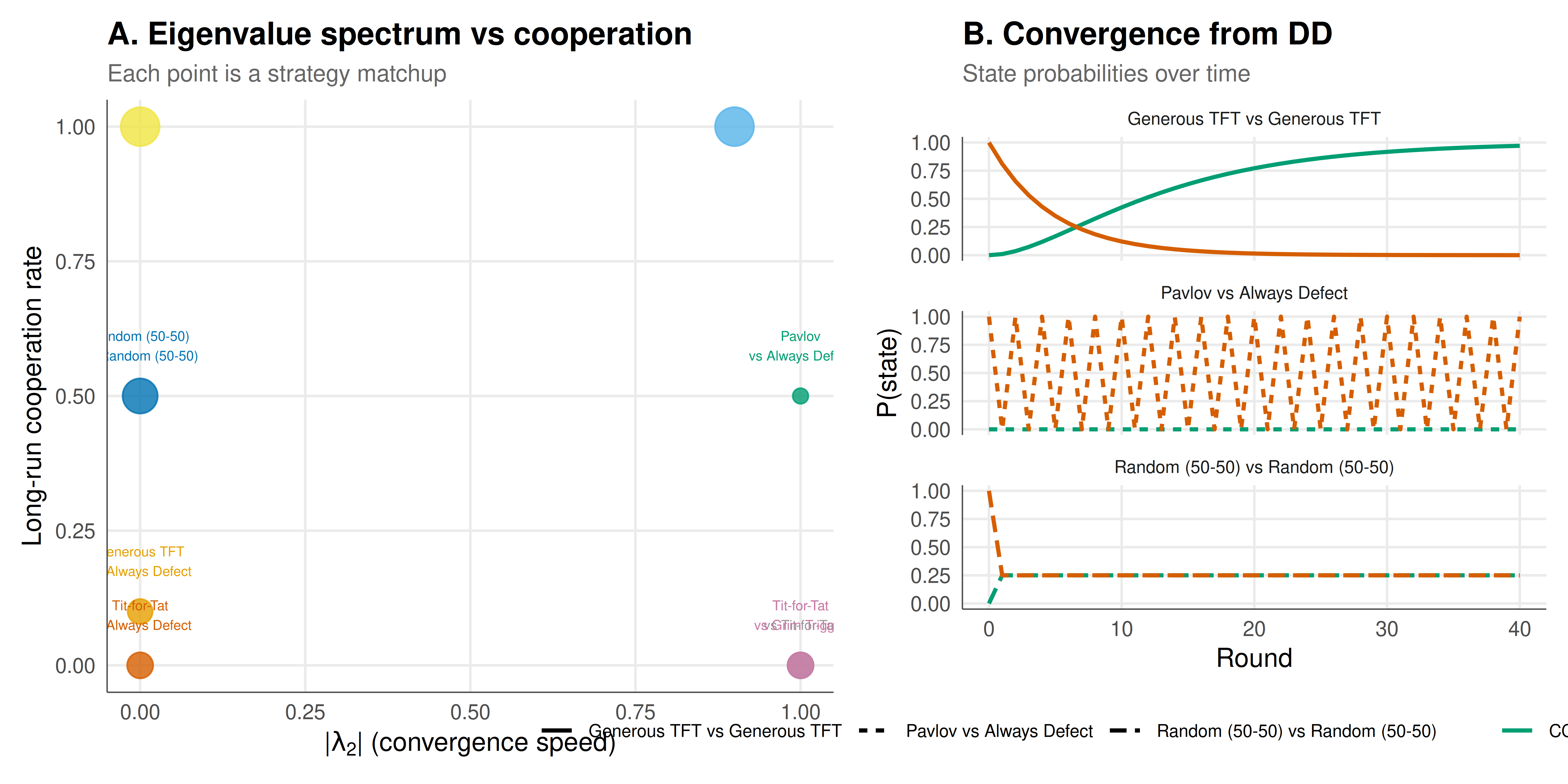
The figure shows the eigenvalue spectra and convergence dynamics for several strategy matchups, illustrating how algebraic properties of the transition matrix determine observable game dynamics.
```{r}
#| label: fig-eigenvalue-static
#| fig-cap: "Figure 1. Left: Second-largest eigenvalue magnitude (|lambda_2|) and long-run cooperation rate for eight strategy matchups in the repeated Prisoner's Dilemma. Larger |lambda_2| means slower convergence; cooperation rate reflects long-run mutual cooperation frequency. Right: Convergence of state probabilities from initial state DD for three matchups, showing how the spectral gap controls convergence speed."
#| dev: [png, pdf]
#| fig-width: 10
#| fig-height: 5
#| dpi: 300
# Panel A: Eigenvalue vs cooperation rate
p_eigen <- ggplot(eigen_summary,
       aes(x = lambda_2, y = coop_rate,
           colour = matchup, size = payoff_p1)) +
  geom_point(alpha = 0.8) +
  geom_text(aes(label = gsub(" vs ", "\nvs ", matchup)),
            size = 2.2, vjust = -1.2, show.legend = FALSE) +
  scale_colour_manual(values = rep(okabe_ito, length.out = nrow(eigen_summary))) +
  scale_size_continuous(range = c(3, 8), name = "P1 payoff") +
  labs(
    title = "A. Eigenvalue spectrum vs cooperation",
    subtitle = "Each point is a strategy matchup",
    x = expression("|" * lambda[2] * "| (convergence speed)"),
    y = "Long-run cooperation rate"
  ) +
  theme_publication() +
  theme(legend.position = "none")

# Panel B: Convergence dynamics
p_conv <- ggplot(conv_all %>% filter(state %in% c("CC", "DD")),
       aes(x = time, y = probability, colour = state, linetype = matchup)) +
  geom_line(linewidth = 0.9) +
  scale_colour_manual(values = okabe_ito[c(3, 6)],
                      labels = c("CC (mutual cooperation)", "DD (mutual defection)")) +
  facet_wrap(~ matchup, ncol = 1, scales = "free_y") +
  labs(
    title = "B. Convergence from DD",
    subtitle = "State probabilities over time",
    x = "Round", y = "P(state)",
    colour = NULL, linetype = NULL
  ) +
  theme_publication() +
  theme(legend.position = "bottom",
        strip.text = element_text(size = 8),
        legend.text = element_text(size = 8))

gridExtra::grid.arrange(p_eigen, p_conv, ncol = 2, widths = c(1.2, 1))
```
## Interactive figure
Explore the eigenvalue analysis interactively. Hover over each matchup to see its full eigenvalue spectrum, spectral gap, mixing time, and long-run payoff.
```{r}
#| label: fig-eigenvalue-interactive
p_int <- ggplot(eigen_summary,
       aes(x = lambda_2, y = coop_rate,
           text = paste0("Matchup: ", matchup,
                         "\n|lambda_2| = ", lambda_2,
                         "\nSpectral gap = ", spectral_gap,
                         "\nMixing time = ", mixing_time,
                         "\nCoop rate = ", coop_rate,
                         "\nP1 payoff = ", payoff_p1),
           size = payoff_p1)) +
  geom_point(aes(colour = matchup), alpha = 0.85) +
  scale_colour_manual(values = rep(okabe_ito, length.out = nrow(eigen_summary))) +
  scale_size_continuous(range = c(4, 10)) +
  labs(
    title = "Eigenvalue spectrum and cooperation in the repeated PD",
    x = "|lambda_2| (larger = slower convergence)",
    y = "Long-run cooperation rate",
    colour = NULL, size = "P1 payoff"
  ) +
  theme_publication() +
  theme(legend.position = "none")

ggplotly(p_int, tooltip = "text") %>%
  config(displaylogo = FALSE) %>%
  layout(legend = list(orientation = "h", y = -0.2))
```
## Interpretation
The eigenvalue analysis reveals a rich structure in the repeated Prisoner's Dilemma that is invisible when examining individual strategy matchups in isolation. Several key insights emerge from the decomposition.
**Spectral gap determines how quickly history is forgotten.** The matchup between Generous TFT and Generous TFT has a moderate spectral gap, meaning that the chain converges to its stationary distribution --- high mutual cooperation --- within about 10-20 rounds. By contrast, matchups involving deterministic strategies (like TFT vs TFT) can have eigenvalue $|\lambda_2| = 1$ or very close to 1, meaning that the initial state permanently influences the trajectory. In the extreme case of TFT vs TFT starting from mutual defection, the chain becomes trapped: if both players defect on round 1, TFT prescribes defection forever. The spectral gap is zero, and there is no "forgetting" of the initial condition. This explains why Generous TFT (which occasionally cooperates even after a defection) outperforms strict TFT in noisy environments: the small forgiveness probability $\epsilon$ creates a positive spectral gap that allows the chain to escape from DD and converge to CC [@axelrod_1984].
**The dominant eigenvalue is always 1.** This is guaranteed by the Perron-Frobenius theorem for irreducible stochastic matrices, and it corresponds to the stationary distribution. For reducible chains (like TFT vs TFT, which has absorbing states), the eigenvalue 1 may have multiplicity greater than 1, indicating multiple stationary distributions --- the long-run outcome depends on the initial state.
**Cooperation rate and payoff are correlated but not identical.** High cooperation rates generally lead to high payoffs, but the relationship is not monotonic because the asymmetric outcomes (CD and DC) contribute differently. In TFT vs Always Defect, the long-run cooperation rate for Player 1 is near zero (Player 1 quickly learns to defect), yielding a payoff close to 1 (mutual defection). In contrast, Pavlov vs Always Defect also produces low cooperation but with a different dynamic pattern.
**Practical implications.** The eigenvalue framework provides a principled way to compare strategies without running Monte Carlo simulations. Given any two memory-one strategies, we can analytically compute the long-run payoff, cooperation rate, and convergence speed in closed form. This makes the approach valuable for evolutionary game theory, where one must evaluate the fitness of strategies against entire populations, and for mechanism design, where the designer wants to predict long-run behaviour under different institutional rules.
## Extensions & related tutorials
The eigenvalue approach generalises naturally to longer memory strategies (larger state spaces), multi-player repeated games (tensor products of transition matrices), and evolutionary dynamics where the strategy population itself evolves.
- [Matrix games and linear algebra](../../linear-algebra-matrix/matrix-games-and-linear-algebra/) --- foundational linear algebra concepts for game theory, including the minimax theorem via linear programming
- [Nash's existence proof](../../history-of-gt-mathematics/nash-equilibrium-original-proof/) --- the fixed-point argument that guarantees equilibria exist; eigenvalue methods help characterise the dynamics *around* equilibria
- [Interactive game theory dashboards](../../visualization-and-communication/interactive-game-theory-dashboards/) --- animated replicator dynamics that can be analysed using the eigenvalue techniques from this tutorial
- [Selten's trembling hand perfection](../../history-of-gt-mathematics/selten-trembling-hand-perfection/) --- equilibrium refinements for perturbed games, where the perturbation structure connects to eigenvalue analysis of perturbed transition matrices
## References
::: {#refs}
:::