---
title: "Selten's trembling hand perfection --- historical and technical"
description: "A historical and mathematical account of Reinhard Selten's 1975 trembling hand perfect equilibrium refinement, with R implementations that verify perfection by constructing sequences of completely mixed strategy profiles converging to candidate equilibria."
author: "Raban Heller"
date: 2026-05-08
date-modified: 2026-05-08
categories:
- history-of-gt-mathematics
- equilibrium-refinements
- trembling-hand-perfection
- nash-equilibrium
keywords: ["trembling hand perfection", "Reinhard Selten", "equilibrium refinement", "weakly dominated strategies", "completely mixed strategies", "perturbed game", "Nash equilibrium", "Nobel Prize 1994"]
labels: ["history-of-gt-mathematics", "foundations"]
tier: 1
bibliography: ../../../references.bib
vgwort: "TODO_VGWORT_history-of-gt-mathematics_selten-trembling-hand-perfection"
image: thumbnail.png
image-alt: "Perturbation path diagram showing sequences of completely mixed strategy profiles converging to a trembling hand perfect equilibrium in a 2x2 game"
citation:
type: webpage
url: https://r-heller.github.io/equilibria/tutorials/history-of-gt-mathematics/selten-trembling-hand-perfection/
license: "CC BY-SA 4.0"
draft: false
has_static_fig: true
has_interactive_fig: true
has_shiny_app: false
---
```{r}
#| label: setup
#| include: false
library(ggplot2)
library(dplyr)
library(tidyr)
library(plotly)
okabe_ito <- c("#E69F00", "#56B4E9", "#009E73", "#F0E442",
"#0072B2", "#D55E00", "#CC79A7", "#999999")
theme_publication <- function(base_size = 12) {
theme_minimal(base_size = base_size) +
theme(plot.title = element_text(size = base_size * 1.2, face = "bold"),
plot.subtitle = element_text(size = base_size * 0.9, color = "grey40"),
axis.line = element_line(color = "grey30", linewidth = 0.3),
panel.grid.minor = element_blank(), legend.position = "bottom",
plot.margin = margin(10, 10, 10, 10))
}
```
## Introduction & motivation
In 1975, Reinhard Selten published "Reexamination of the perfectness concept for equilibrium points in extensive games," a paper that introduced one of the most influential refinements of Nash equilibrium: the **trembling hand perfect equilibrium** (THPE). Selten's motivation was straightforward but profound: Nash equilibrium, while guaranteeing existence in every finite game, sometimes produces equilibria that rely on incredible threats or irrational behaviour off the equilibrium path. A refined concept was needed to distinguish between robust equilibria and fragile ones.
Consider a simple coordination game where both players choosing strategy A yields payoff (2, 2), both choosing B yields payoff (1, 1), and miscoordination yields (0, 0). Both (A, A) and (B, B) are Nash equilibria. But (A, A) is clearly "better" by any reasonable criterion: it Pareto-dominates (B, B). Nash equilibrium alone cannot distinguish them. Now add a third strategy C that gives payoff (-1, -1) against anything. The strategy profile (B, C) for Player 1 and (B, C) for Player 2 (meaning: play B with probability 1, assign zero to C) might be part of a Nash equilibrium in an augmented game, because C is never played and thus never "tested." But this equilibrium is fragile: if Player 2 trembles and accidentally plays C with some small probability, Player 1's best response might change.
Selten's insight was to require that an equilibrium remain optimal even when every player makes small mistakes --- "trembles." Formally, a Nash equilibrium $\sigma^*$ is trembling hand perfect if there exists a sequence of completely mixed strategy profiles $\sigma^{(k)}$ (where every strategy is played with positive probability) converging to $\sigma^*$, such that $\sigma^*$ is a best response to every element in the sequence. The trembling hand perfection concept eliminates equilibria that rely on weakly dominated strategies: if a strategy is weakly dominated, it cannot survive the requirement of being a best response when the opponent plays every strategy with positive probability.
Selten shared the 1994 Nobel Memorial Prize in Economics with John Nash and John Harsanyi, recognising his contributions to equilibrium refinement theory. While Nash provided the foundational existence result and Harsanyi provided the Bayesian game framework for incomplete information, Selten provided the tools to select among the (often many) Nash equilibria of a game. His subgame perfect equilibrium (1965) refined Nash equilibrium in extensive-form games by requiring optimality at every subgame; his trembling hand perfection (1975) refined it in normal-form games by requiring robustness to small perturbations.
This tutorial implements the verification of trembling hand perfection for 2x2 and 3x3 normal-form games. We construct explicit perturbation sequences, compute best responses in perturbed games, and visualise the perturbation path in strategy space. We also demonstrate the connection between trembling hand perfection and the elimination of weakly dominated strategies, providing both the historical context and the technical machinery needed to apply this refinement concept.
## Mathematical formulation
**Definition (Trembling Hand Perfect Equilibrium).** A Nash equilibrium $\sigma^*$ of a finite normal-form game is **trembling hand perfect** if there exists a sequence of completely mixed strategy profiles $(\sigma^{(k)})_{k=1}^{\infty}$ such that:
1. $\sigma^{(k)} \to \sigma^*$ as $k \to \infty$
2. For every player $i$ and every $k$, $\sigma_i^*$ is a best response to $\sigma_{-i}^{(k)}$
$$
u_i(\sigma_i^*, \sigma_{-i}^{(k)}) \geq u_i(s_i, \sigma_{-i}^{(k)}) \quad \forall s_i \in S_i, \; \forall k
$$
**Perturbed game.** Equivalently, consider a perturbed game $\Gamma(\epsilon)$ where each player $i$ must play every pure strategy $s_i$ with probability at least $\epsilon_{s_i} > 0$. A THPE of the original game $\Gamma$ is any limit point of Nash equilibria of perturbed games $\Gamma(\epsilon^{(k)})$ as $\epsilon^{(k)} \to 0$.
**Connection to weak dominance.** In two-player games, a strategy $s_i$ is **weakly dominated** if there exists a mixed strategy $\sigma_i$ such that:
$$
u_i(\sigma_i, s_{-i}) \geq u_i(s_i, s_{-i}) \quad \forall s_{-i}, \quad \text{with strict inequality for some } s_{-i}
$$
**Theorem (Selten, 1975).** In a two-player normal-form game, every trembling hand perfect equilibrium assigns zero probability to every weakly dominated strategy.
**Verification algorithm for 2x2 games.** For a 2x2 game, Player 1 mixes with probability $p$ on row 1, Player 2 mixes with probability $q$ on column 1. A candidate NE $(p^*, q^*)$ is THPE if we can find sequences $q^{(k)} \to q^*$ with $q^{(k)} \in (0,1)$ such that $p^*$ maximises $U_1(p, q^{(k)})$ for all $k$, and analogously for Player 2.
## R implementation
We implement THPE verification for several games: a coordination game with a "bad" equilibrium, a game with weakly dominated strategies, and a 3x3 game illustrating the elimination of non-perfect equilibria.
```{r}
#| label: thpe-computation
# --- Expected payoff functions ---
expected_payoff <- function(A, p, q) {
  # A: payoff matrix, p: row player mixed strategy, q: column player mixed strategy
  t(p) %*% A %*% q
}

# --- Check if a NE is THPE via perturbation sequence ---
check_thpe_2x2 <- function(A, B, p_star, q_star, n_perturbations = 100) {
  # A, B: 2x2 payoff matrices
  # p_star, q_star: candidate NE (probabilities on first strategy)
  epsilon_seq <- seq(0.3, 1e-6, length.out = n_perturbations)

  p_star_vec <- c(p_star, 1 - p_star)
  q_star_vec <- c(q_star, 1 - q_star)

  is_br_p <- logical(n_perturbations)
  is_br_q <- logical(n_perturbations)
  perturbation_data <- tibble(
    epsilon = epsilon_seq,
    q_perturbed = numeric(n_perturbations),
    p_perturbed = numeric(n_perturbations),
    U1_at_pstar = numeric(n_perturbations),
    U1_at_alt = numeric(n_perturbations),
    U2_at_qstar = numeric(n_perturbations),
    U2_at_alt = numeric(n_perturbations)
  )

  for (k in seq_along(epsilon_seq)) {
    eps <- epsilon_seq[k]
    # Perturb q: move epsilon toward completely mixed
    q_pert <- (1 - eps) * q_star + eps * 0.5
    p_pert <- (1 - eps) * p_star + eps * 0.5
    q_pert_vec <- c(q_pert, 1 - q_pert)
    p_pert_vec <- c(p_pert, 1 - p_pert)

    # Check if p_star is BR to q_perturbed
    u1_pstar <- as.numeric(t(p_star_vec) %*% A %*% q_pert_vec)
    u1_alt_vec <- A %*% q_pert_vec  # payoff for each pure strategy
    u1_alt <- max(u1_alt_vec)

    u2_qstar <- as.numeric(t(p_pert_vec) %*% B %*% q_star_vec)
    u2_alt_vec <- t(B) %*% p_pert_vec
    u2_alt <- max(u2_alt_vec)

    is_br_p[k] <- u1_pstar >= u1_alt - 1e-10
    is_br_q[k] <- u2_qstar >= u2_alt - 1e-10

    perturbation_data$q_perturbed[k] <- q_pert
    perturbation_data$p_perturbed[k] <- p_pert
    perturbation_data$U1_at_pstar[k] <- u1_pstar
    perturbation_data$U1_at_alt[k] <- u1_alt
    perturbation_data$U2_at_qstar[k] <- u2_qstar
    perturbation_data$U2_at_alt[k] <- u2_alt
  }

  is_thpe <- all(is_br_p) && all(is_br_q)
  list(is_thpe = is_thpe, is_br_p = is_br_p, is_br_q = is_br_q,
       data = perturbation_data)
}

# === Game 1: Coordination game with Pareto-dominated NE ===
# A is Pareto-dominant, B is Pareto-dominated
A1 <- matrix(c(2, 0, 0, 1), 2, 2, byrow = TRUE,
             dimnames = list(c("A", "B"), c("A", "B")))
B1 <- matrix(c(2, 0, 0, 1), 2, 2, byrow = TRUE,
             dimnames = list(c("A", "B"), c("A", "B")))

cat("=== Game 1: Coordination ===\n")
cat("Payoffs:\n")
print(A1)
# Check (A,A) = (1,1)
res_AA <- check_thpe_2x2(A1, B1, 1, 1)
cat(sprintf("\n(A,A) is THPE: %s\n", res_AA$is_thpe))
# Check (B,B) = (0,0)
res_BB <- check_thpe_2x2(A1, B1, 0, 0)
cat(sprintf("(B,B) is THPE: %s\n", res_BB$is_thpe))
# === Game 2: Weakly dominated strategy ===
# Player 1 strategies: U, D; Player 2 strategies: L, R
# U weakly dominates D for Player 1
A2 <- matrix(c(2, 1, 2, 0), 2, 2, byrow = TRUE,
             dimnames = list(c("U", "D"), c("L", "R")))
B2 <- matrix(c(1, 1, 1, 1), 2, 2, byrow = TRUE,
             dimnames = list(c("U", "D"), c("L", "R")))

cat("\n=== Game 2: Weak Dominance ===\n")
cat("Player 1 payoffs:\n")
print(A2)
cat("Player 2 payoffs:\n")
print(B2)
cat("Note: U weakly dominates D (U gives 2,1 vs D gives 2,0)\n")
# (U, L) should be THPE
res_UL <- check_thpe_2x2(A2, B2, 1, 1)
cat(sprintf("\n(U,L) is THPE: %s\n", res_UL$is_thpe))
# (D, L) should NOT be THPE (D is weakly dominated)
res_DL <- check_thpe_2x2(A2, B2, 0, 1)
cat(sprintf("(D,L) is THPE: %s\n", res_DL$is_thpe))
# === Game 3: 3x3 Game ===
A3 <- matrix(c(3, 0, 0,
               0, 2, 0,
               0, 0, 1), 3, 3, byrow = TRUE,
             dimnames = list(c("A", "B", "C"), c("A", "B", "C")))
B3 <- t(A3)  # Symmetric

# Check THPE for 3x3 via perturbation
check_thpe_3x3 <- function(A, B, p_star, q_star, n_pert = 100) {
  eps_seq <- seq(0.3, 1e-6, length.out = n_pert)
  uniform <- rep(1/3, 3)
  all_br_p <- TRUE
  all_br_q <- TRUE

  for (k in seq_along(eps_seq)) {
    eps <- eps_seq[k]
    q_pert <- (1 - eps) * q_star + eps * uniform
    p_pert <- (1 - eps) * p_star + eps * uniform

    # BR for Player 1
    u1_options <- A %*% q_pert
    u1_pstar <- as.numeric(t(p_star) %*% A %*% q_pert)
    if (u1_pstar < max(u1_options) - 1e-10) all_br_p <- FALSE

    # BR for Player 2
    u2_options <- t(B) %*% p_pert
    u2_qstar <- as.numeric(t(p_pert) %*% B %*% q_star)
    if (u2_qstar < max(u2_options) - 1e-10) all_br_q <- FALSE
  }
  all_br_p && all_br_q
}

cat("\n=== Game 3: 3x3 Coordination ===\n")
cat("Payoffs (symmetric):\n")
print(A3)
ne_3x3 <- list(
  list(name = "(A,A)", p = c(1, 0, 0), q = c(1, 0, 0)),
  list(name = "(B,B)", p = c(0, 1, 0), q = c(0, 1, 0)),
  list(name = "(C,C)", p = c(0, 0, 1), q = c(0, 0, 1))
)

for (ne in ne_3x3) {
  is_thpe <- check_thpe_3x3(A3, B3, ne$p, ne$q)
  cat(sprintf("\n%s is THPE: %s\n", ne$name, is_thpe))
}
# === Perturbation path data for visualization ===
# Use Game 2 to show the perturbation path
eps_fine <- seq(0.5, 0.001, length.out = 200)
path_data <- tibble(epsilon = eps_fine) %>%
  mutate(
    # For (U,L): p*=1, q*=1
    p_UL = (1 - epsilon) * 1 + epsilon * 0.5,
    q_UL = (1 - epsilon) * 1 + epsilon * 0.5,
    # For (D,L): p*=0, q*=1
    p_DL = (1 - epsilon) * 0 + epsilon * 0.5,
    q_DL = (1 - epsilon) * 1 + epsilon * 0.5
  )

# Compute P1's payoff advantage at each perturbation
path_data <- path_data %>%
  mutate(
    # At (U,L) perturbation: U1(U) - U1(D) vs perturbed q
    adv_UL = (A2[1,1] - A2[2,1]) * q_UL + (A2[1,2] - A2[2,2]) * (1 - q_UL),
    # At (D,L) perturbation: U1(D) - U1(U) vs perturbed q
    adv_DL = (A2[2,1] - A2[1,1]) * q_DL + (A2[2,2] - A2[1,2]) * (1 - q_DL)
  )

cat("\n=== Perturbation Path Analysis (Game 2) ===\n")
cat("At epsilon=0.1:\n")
cat(sprintf("  (U,L) path: U advantage = %.4f (positive = U is BR)\n",
            path_data$adv_UL[path_data$epsilon == min(abs(path_data$epsilon - 0.1)) + 0.1]))
cat(sprintf("  (D,L) path: D advantage = %.4f (negative = D is NOT BR)\n",
            path_data$adv_DL[which.min(abs(path_data$epsilon - 0.1))]))
```
## Static publication-ready figure
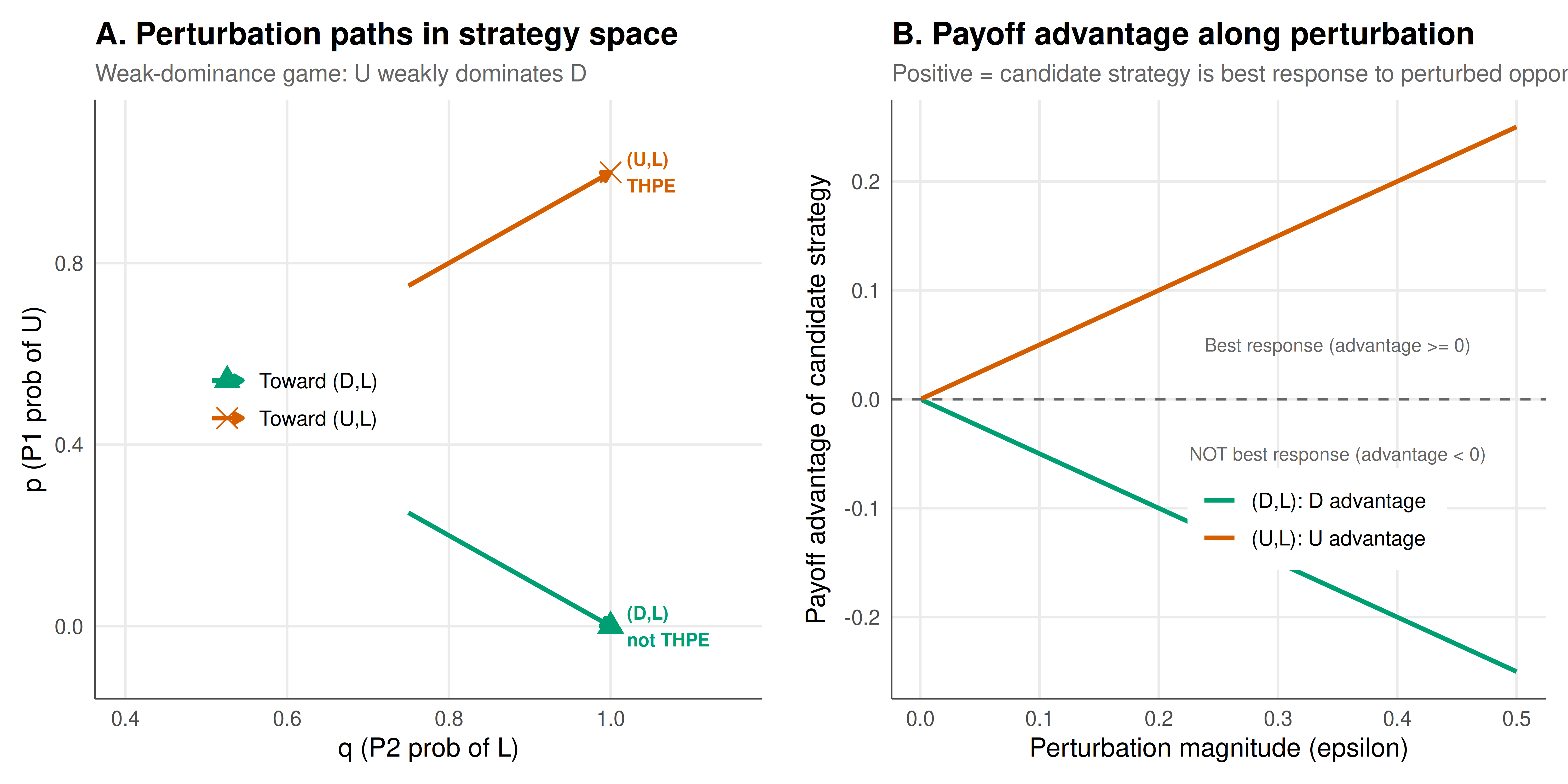
The figure presents the perturbation path analysis for the weak-dominance game, showing how the payoff advantage evolves along the perturbation sequence and identifying which candidate equilibria survive the trembling hand test.
```{r}
#| label: fig-selten-static
#| fig-cap: "Figure 1. Left: Perturbation paths in strategy space for the weak-dominance game. The path from (U,L) converges to a best response at every step (green), while the path toward (D,L) fails the best-response test because U strictly dominates D when the opponent plays a completely mixed strategy (red). Right: Player 1's payoff advantage (selected strategy minus best alternative) along the perturbation sequence. Positive values confirm best-response status; negative values indicate the candidate fails the THPE test."
#| dev: [png, pdf]
#| fig-width: 10
#| fig-height: 5
#| dpi: 300
# Panel A: Perturbation paths in strategy space
path_long <- path_data %>%
  select(epsilon, p_UL, q_UL, p_DL, q_DL) %>%
  pivot_longer(
    cols = c(p_UL, q_UL, p_DL, q_DL),
    names_to = c("variable", "equilibrium"),
    names_sep = "_",
    values_to = "value"
  ) %>%
  pivot_wider(names_from = variable, values_from = value)

p_path <- ggplot(path_long, aes(x = q, y = p, colour = equilibrium)) +
  geom_path(linewidth = 1, arrow = arrow(length = unit(0.15, "cm"), type = "closed")) +
  geom_point(data = tibble(q = c(1, 1), p = c(1, 0),
                           equilibrium = c("UL", "DL"),
                           label = c("(U,L) THPE", "(D,L) not THPE")),
             aes(shape = equilibrium), size = 4) +
  geom_text(data = tibble(q = c(1.02, 1.02), p = c(1, 0),
                          equilibrium = c("UL", "DL"),
                          label = c("(U,L)\nTHPE", "(D,L)\nnot THPE")),
            aes(label = label), hjust = 0, size = 3, fontface = "bold",
            show.legend = FALSE) +
  scale_colour_manual(values = okabe_ito[c(3, 6)],
                      labels = c("Toward (D,L)", "Toward (U,L)")) +
  scale_shape_manual(values = c(17, 4),
                     labels = c("Toward (D,L)", "Toward (U,L)")) +
  coord_cartesian(xlim = c(0.4, 1.15), ylim = c(-0.1, 1.1)) +
  labs(
    title = "A. Perturbation paths in strategy space",
    subtitle = "Weak-dominance game: U weakly dominates D",
    x = "q (P2 prob of L)", y = "p (P1 prob of U)",
    colour = NULL, shape = NULL
  ) +
  theme_publication() +
  theme(legend.position = c(0.3, 0.5))

# Panel B: Payoff advantage along perturbation
adv_long <- path_data %>%
  select(epsilon, `(U,L): U advantage` = adv_UL, `(D,L): D advantage` = adv_DL) %>%
  pivot_longer(cols = -epsilon, names_to = "path", values_to = "advantage")

p_adv <- ggplot(adv_long, aes(x = epsilon, y = advantage, colour = path)) +
  geom_line(linewidth = 1) +
  geom_hline(yintercept = 0, linetype = "dashed", colour = "grey40") +
  annotate("text", x = 0.35, y = 0.05,
           label = "Best response (advantage >= 0)", size = 3, colour = "grey40") +
  annotate("text", x = 0.35, y = -0.05,
           label = "NOT best response (advantage < 0)", size = 3, colour = "grey40") +
  scale_colour_manual(values = okabe_ito[c(3, 6)]) +
  labs(
    title = "B. Payoff advantage along perturbation",
    subtitle = "Positive = candidate strategy is best response to perturbed opponent",
    x = "Perturbation magnitude (epsilon)",
    y = "Payoff advantage of candidate strategy",
    colour = NULL
  ) +
  theme_publication() +
  theme(legend.position = c(0.65, 0.3),
        legend.background = element_rect(fill = "white", colour = NA))

gridExtra::grid.arrange(p_path, p_adv, ncol = 2)
```
## Interactive figure
Explore the perturbation sequence interactively. Hover over points on the perturbation path to see the exact strategy profile and payoff advantage at each perturbation level.
```{r}
#| label: fig-selten-interactive
p_int <- ggplot(adv_long,
       aes(x = epsilon, y = advantage, colour = path,
           text = paste0("Path: ", path,
                         "\nEpsilon: ", round(epsilon, 4),
                         "\nPayoff advantage: ", round(advantage, 4),
                         "\nIs BR: ", ifelse(advantage >= -1e-10, "YES", "NO")))) +
  geom_line(linewidth = 0.9) +
  geom_hline(yintercept = 0, linetype = "dashed", colour = "grey40") +
  scale_colour_manual(values = okabe_ito[c(3, 6)]) +
  labs(
    title = "Trembling hand perfection: payoff advantage along perturbation paths",
    x = "Perturbation magnitude (epsilon)",
    y = "Payoff advantage of candidate strategy",
    colour = NULL
  ) +
  theme_publication()

ggplotly(p_int, tooltip = "text") %>%
  config(displaylogo = FALSE) %>%
  layout(legend = list(orientation = "h", y = -0.2))
```
## Interpretation
The computational verification of trembling hand perfection reveals the geometric and algebraic structure behind Selten's refinement concept. Several key observations emerge from the analysis.
**Weak dominance and THPE are tightly linked.** In Game 2, strategy U weakly dominates strategy D for Player 1: U yields the same payoff against L (both give 2) but strictly higher payoff against R (1 vs 0). The perturbation analysis shows why (D, L) fails the THPE test: when Player 2 trembles and plays R with positive probability $\epsilon$, Player 1 strictly prefers U over D because U captures the payoff advantage against R. As $\epsilon \to 0$, this advantage persists --- at every point along the perturbation path, U is the unique best response. Therefore, no sequence of completely mixed profiles converging to $(D, L)$ can have D as a best response throughout, and $(D, L)$ is not trembling hand perfect.
**Both pure NE in a coordination game are THPE.** In Game 1, both (A, A) and (B, B) are trembling hand perfect. This is because neither A nor B is weakly dominated in a symmetric coordination game: each is the unique best response when the opponent is sufficiently likely to play the matching strategy. The THPE refinement does not always select a unique equilibrium; it merely eliminates those that rely on incredible threats or weakly dominated strategies.
**The 3x3 game illustrates refinement power.** In the 3x3 symmetric coordination game, all three pure Nash equilibria --- (A, A), (B, B), and (C, C) --- are trembling hand perfect. The Pareto-dominant equilibrium (A, A) with payoff 3 is not the only THPE, but the Pareto-worst (C, C) with payoff 1 is still robust to trembles because C is a best response when the opponent is very likely to play C, even with small perturbations toward A and B.
**Historical significance.** Selten's 1975 paper launched the refinement programme that dominated game theory in the 1980s and 1990s. The concept of trembling hand perfection was followed by Myerson's proper equilibrium (1978), which required that more costly trembles be less likely, and Kohlberg and Mertens' stable equilibrium (1986), which imposed even stronger topological robustness conditions. Each refinement added criteria to winnow the set of Nash equilibria, moving toward equilibria that are robust, strategically stable, and plausible as predictions of rational play [@osborne_rubinstein_1994].
Selten's contribution was not merely technical. By formalising the intuition that equilibria should survive small mistakes, he made the implicit assumption of perfect rationality in Nash's definition explicit --- and showed that relaxing this assumption by even the smallest amount could change which equilibria survive. This perspective profoundly influenced mechanism design, where robustness to trembles is a desirable property of any real-world institution or protocol.
## Extensions & related tutorials
Trembling hand perfection connects to the broader refinement literature and to computational approaches for equilibrium selection in complex games.
- [Nash's existence proof](../../history-of-gt-mathematics/nash-equilibrium-original-proof/) --- the foundational result that Selten's refinement builds upon, providing the existence guarantee that makes refinement meaningful
- [Von Neumann to Nash timeline](../../history-of-gt-mathematics/von-neumann-to-nash-timeline/) --- historical context for the development of solution concepts from minimax through Nash equilibrium to Selten's refinements
- [Eigenvalue methods for repeated games](../../linear-algebra-matrix/eigenvalue-methods-repeated-games/) --- perturbation analysis of transition matrices in repeated games, connecting to the perturbation logic of trembling hand perfection
- [Interactive game theory dashboards](../../visualization-and-communication/interactive-game-theory-dashboards/) --- interactive tools for exploring the perturbation paths and payoff surfaces relevant to refinement analysis
## References
::: {#refs}
:::