---
title: "Interactive game theory dashboards with plotly"
description: "Build advanced interactive visualisations for game theory using plotly in R: animated replicator dynamics, hover-enabled payoff matrices, linked strategy-payoff views, and 3D expected-payoff surfaces over the mixed-strategy simplex."
author: "Raban Heller"
date: 2026-05-08
date-modified: 2026-05-08
categories:
- visualization-and-communication
- plotly
- interactive-visualization
- replicator-dynamics
keywords: ["plotly", "interactive visualization", "replicator dynamics", "payoff matrix", "3D surface", "game theory dashboard", "mixed strategy", "ggplotly"]
labels: ["visualization-and-communication", "tools"]
tier: 1
bibliography: ../../../references.bib
vgwort: "TODO_VGWORT_visualization-and-communication_interactive-game-theory-dashboards"
image: thumbnail.png
image-alt: "Screenshot of an interactive plotly dashboard showing a 3D expected-payoff surface over the mixed-strategy space for a 2x2 game"
citation:
type: webpage
url: https://r-heller.github.io/equilibria/tutorials/visualization-and-communication/interactive-game-theory-dashboards/
license: "CC BY-SA 4.0"
draft: false
has_static_fig: true
has_interactive_fig: true
has_shiny_app: false
---
```{r}
#| label: setup
#| include: false
library(ggplot2)
library(dplyr)
library(tidyr)
library(plotly)
okabe_ito <- c("#E69F00", "#56B4E9", "#009E73", "#F0E442",
"#0072B2", "#D55E00", "#CC79A7", "#999999")
theme_publication <- function(base_size = 12) {
theme_minimal(base_size = base_size) +
theme(plot.title = element_text(size = base_size * 1.2, face = "bold"),
plot.subtitle = element_text(size = base_size * 0.9, color = "grey40"),
axis.line = element_line(color = "grey30", linewidth = 0.3),
panel.grid.minor = element_blank(), legend.position = "bottom",
plot.margin = margin(10, 10, 10, 10))
}
```
## Introduction & motivation
Game theory generates some of the richest visual structures in applied mathematics: payoff matrices with colour-coded best responses, trajectory fields showing how populations of strategies evolve over time, simplicial representations of mixed-strategy spaces, and surfaces of expected payoffs over multi-dimensional strategy sets. Yet most textbook figures are static, forcing the reader to mentally interpolate between a few selected parameter values or trace dynamics by eye. Interactive visualisation transforms these figures from passive illustrations into active analytical tools.
The `plotly` package in R --- whether used directly via `plot_ly()` or by converting `ggplot2` objects with `ggplotly()` --- provides a powerful framework for building interactive game theory dashboards. Hover tooltips can reveal exact payoff values and highlight best responses in a normal-form game matrix. Animation frames can show the temporal evolution of replicator dynamics, allowing the viewer to pause, scrub forward, and inspect the state at any time step. Linked brushing (via `highlight()`) can connect a view of the strategy space to a view of the payoff space, so that selecting a trajectory in one panel highlights the corresponding payoffs in the other. And 3D surface plots can display the full expected-payoff landscape over the mixed-strategy simplex, letting the viewer rotate, zoom, and identify saddle points, maxima, and equilibria from any angle.
This tutorial teaches advanced `plotly` techniques through four concrete game theory examples. Each example introduces a different `plotly` capability --- hover interactivity, animation, linked views, and 3D surfaces --- while simultaneously building substantive game-theoretic intuition. The goal is twofold: to equip the reader with the technical skills to build publication-quality interactive figures, and to demonstrate how interactivity itself deepens understanding of strategic concepts.
We assume familiarity with basic `ggplot2` (see the publication-ready ggplot theme tutorial elsewhere on this site) and basic game theory concepts (Nash equilibrium, mixed strategies, replicator dynamics). All interactive figures in this tutorial are self-contained HTML widgets that work without a server, making them suitable for Quarto documents, websites, and presentations.
The four dashboard components we build are: (1) an interactive payoff matrix for the Prisoner's Dilemma with best-response highlighting, (2) an animated trajectory of replicator dynamics in a Rock-Paper-Scissors game, (3) linked brushing connecting the Hawk-Dove strategy space to the payoff space, and (4) a 3D surface of Player 1's expected payoff over the full mixed-strategy space of a Battle of the Sexes game. Together, these demonstrate the core `plotly` features most relevant to game theory visualisation.
## Mathematical formulation
**Normal-form games.** A two-player game is defined by payoff matrices $A$ (Player 1) and $B$ (Player 2), each of dimension $m \times n$. When Player 1 plays row $i$ and Player 2 plays column $j$, the payoffs are $(A_{ij}, B_{ij})$.
**Mixed strategies.** Player 1's mixed strategy $\mathbf{p} = (p_1, \dots, p_m)$ lies on the simplex $\Delta^{m-1} = \{\mathbf{p} \in \mathbb{R}^m : p_i \geq 0, \sum p_i = 1\}$. Player 1's expected payoff given strategies $\mathbf{p}$ and $\mathbf{q}$ is:
$$
U_1(\mathbf{p}, \mathbf{q}) = \mathbf{p}^\top A \mathbf{q} = \sum_{i=1}^{m} \sum_{j=1}^{n} p_i \, A_{ij} \, q_j
$$
**Replicator dynamics.** In a symmetric game with payoff matrix $A$, the population share $x_i$ of strategy $i$ evolves according to:
$$
\dot{x}_i = x_i \left[ (A\mathbf{x})_i - \mathbf{x}^\top A \mathbf{x} \right]
$$
where $(A\mathbf{x})_i$ is the fitness of strategy $i$ against population $\mathbf{x}$, and $\mathbf{x}^\top A \mathbf{x}$ is the average population fitness [@taylor_jonker_1978].
**Best response.** Strategy $i$ is a best response for Player 1 against Player 2's strategy $\mathbf{q}$ if:
$$
(A\mathbf{q})_i \geq (A\mathbf{q})_k \quad \forall k
$$
In a payoff matrix display, best responses are the maximum entries in each column (for Player 1) and each row (for Player 2).
## R implementation
We build the four dashboard components sequentially, starting with the data generation and computation, then constructing each interactive figure.
```{r}
#| label: dashboard-computation
# === Component 1: Interactive Payoff Matrix ===
# Prisoner's Dilemma
pd_A <- matrix(c(3, 0, 5, 1), 2, 2, byrow = TRUE,
               dimnames = list(c("Cooperate", "Defect"), c("Cooperate", "Defect")))
pd_B <- matrix(c(3, 5, 0, 1), 2, 2, byrow = TRUE,
               dimnames = list(c("Cooperate", "Defect"), c("Cooperate", "Defect")))

# Build hover text matrix
payoff_text <- matrix("", 2, 2)
for (i in 1:2) {
  for (j in 1:2) {
    is_br1 <- pd_A[i, j] == max(pd_A[, j])
    is_br2 <- pd_B[i, j] == max(pd_B[i, ])
    br_tag <- ""
    if (is_br1 && is_br2) br_tag <- " [NE]"
    else if (is_br1) br_tag <- " [BR for P1]"
    else if (is_br2) br_tag <- " [BR for P2]"
    payoff_text[i, j] <- paste0(
      "P1: ", rownames(pd_A)[i], ", P2: ", colnames(pd_A)[j],
      "\nPayoff P1: ", pd_A[i, j], ", Payoff P2: ", pd_B[i, j],
      br_tag
    )
  }
}

# Payoff matrix data frame for heatmap
pm_df <- expand.grid(P1 = rownames(pd_A), P2 = colnames(pd_A)) %>%
  mutate(
    payoff_p1 = as.vector(pd_A),
    payoff_p2 = as.vector(pd_B),
    total = payoff_p1 + payoff_p2,
    hover = as.vector(payoff_text),
    label = paste0("(", payoff_p1, ", ", payoff_p2, ")")
  )

cat("=== Prisoner's Dilemma Payoff Matrix ===\n")
cat("Player 1 payoffs:\n")
print(pd_A)
cat("\nPlayer 2 payoffs:\n")
print(pd_B)
# === Component 2: Animated Replicator Dynamics (Rock-Paper-Scissors) ===
rps_A <- matrix(c(0, -1, 1, 1, 0, -1, -1, 1, 0), 3, 3, byrow = TRUE)

replicator_step <- function(x, A, dt = 0.02) {
  Ax <- as.vector(A %*% x)
  avg_fitness <- sum(x * Ax)
  x_new <- x + dt * x * (Ax - avg_fitness)
  x_new <- pmax(x_new, 1e-10)
  x_new / sum(x_new)
}

# Simulate multiple trajectories
set.seed(42)
n_traj <- 5
n_steps <- 300
dt <- 0.02

traj_data <- list()
for (tr in 1:n_traj) {
  x <- runif(3)
  x <- x / sum(x)
  traj <- matrix(0, n_steps + 1, 3)
  traj[1, ] <- x
  for (t in 1:n_steps) {
    x <- replicator_step(x, rps_A, dt)
    traj[t + 1, ] <- x
  }
  traj_df <- as.data.frame(traj) %>%
    setNames(c("Rock", "Paper", "Scissors")) %>%
    mutate(time = 0:n_steps, trajectory = paste0("Traj ", tr))
  traj_data[[tr]] <- traj_df
}

rps_long <- bind_rows(traj_data) %>%
  pivot_longer(cols = c(Rock, Paper, Scissors),
               names_to = "strategy", values_to = "share")

cat("\n=== Replicator Dynamics: RPS ===\n")
cat("Payoff matrix (Rock-Paper-Scissors):\n")
print(rps_A)
cat("\nFinal state of trajectory 1:\n")
final <- traj_data[[1]] %>% filter(time == n_steps)
cat(sprintf("  Rock: %.4f, Paper: %.4f, Scissors: %.4f\n",
            final$Rock, final$Paper, final$Scissors))
# === Component 3: Hawk-Dove Strategy & Payoff Spaces ===
# Hawk-Dove: payoff matrix parameterised by V (value) and C (cost)
V <- 4
C <- 6
hd_A <- matrix(c((V - C) / 2, V, 0, V / 2), 2, 2, byrow = TRUE,
               dimnames = list(c("Hawk", "Dove"), c("Hawk", "Dove")))

# Strategy space: p = prob(Hawk) for each player
p_grid <- seq(0, 1, length.out = 80)
hd_grid <- expand.grid(p1 = p_grid, p2 = p_grid) %>%
  as_tibble() %>%
  mutate(
    U1 = p1 * p2 * hd_A[1,1] + p1 * (1 - p2) * hd_A[1,2] +
         (1 - p1) * p2 * hd_A[2,1] + (1 - p1) * (1 - p2) * hd_A[2,2],
    U2 = p2 * p1 * hd_A[1,1] + p2 * (1 - p1) * hd_A[1,2] +
         (1 - p2) * p1 * hd_A[2,1] + (1 - p2) * (1 - p1) * hd_A[2,2],
    total_welfare = U1 + U2
  )

# Nash equilibrium: p* = V/C for symmetric game
p_star <- V / C
cat("\n=== Hawk-Dove Game (V=4, C=6) ===\n")
cat("Payoff matrix:\n")
print(hd_A)
cat(sprintf("\nMixed NE: p* = V/C = %.4f\n", p_star))
# === Component 4: 3D Surface (Battle of the Sexes) ===
bos_A <- matrix(c(3, 0, 0, 2), 2, 2, byrow = TRUE)
bos_B <- matrix(c(2, 0, 0, 3), 2, 2, byrow = TRUE)

p_seq <- seq(0, 1, length.out = 60)
q_seq <- seq(0, 1, length.out = 60)
bos_surface <- expand.grid(p = p_seq, q = q_seq) %>%
  as_tibble() %>%
  mutate(
    U1 = p * q * bos_A[1,1] + p * (1 - q) * bos_A[1,2] +
         (1 - p) * q * bos_A[2,1] + (1 - p) * (1 - q) * bos_A[2,2],
    U2 = p * q * bos_B[1,1] + p * (1 - q) * bos_B[1,2] +
         (1 - p) * q * bos_B[2,1] + (1 - p) * (1 - q) * bos_B[2,2]
  )

# NE points for Battle of the Sexes
# Pure NE: (1,1) and (0,0); Mixed NE: p*=3/5, q*=2/5
bos_ne <- tibble(
  p = c(1, 0, 3/5), q = c(1, 0, 2/5),
  label = c("Pure NE (Opera, Opera)", "Pure NE (Football, Football)",
            "Mixed NE (3/5, 2/5)")
) %>%
  mutate(
    U1 = p * q * bos_A[1,1] + p * (1 - q) * bos_A[1,2] +
         (1 - p) * q * bos_A[2,1] + (1 - p) * (1 - q) * bos_A[2,2]
  )

cat("\n=== Battle of the Sexes ===\n")
cat("Nash equilibria:\n")
for (i in 1:nrow(bos_ne)) {
  cat(sprintf("  %s: p=%.2f, q=%.2f, U1=%.3f\n",
              bos_ne$label[i], bos_ne$p[i], bos_ne$q[i], bos_ne$U1[i]))
}
```
## Static publication-ready figure
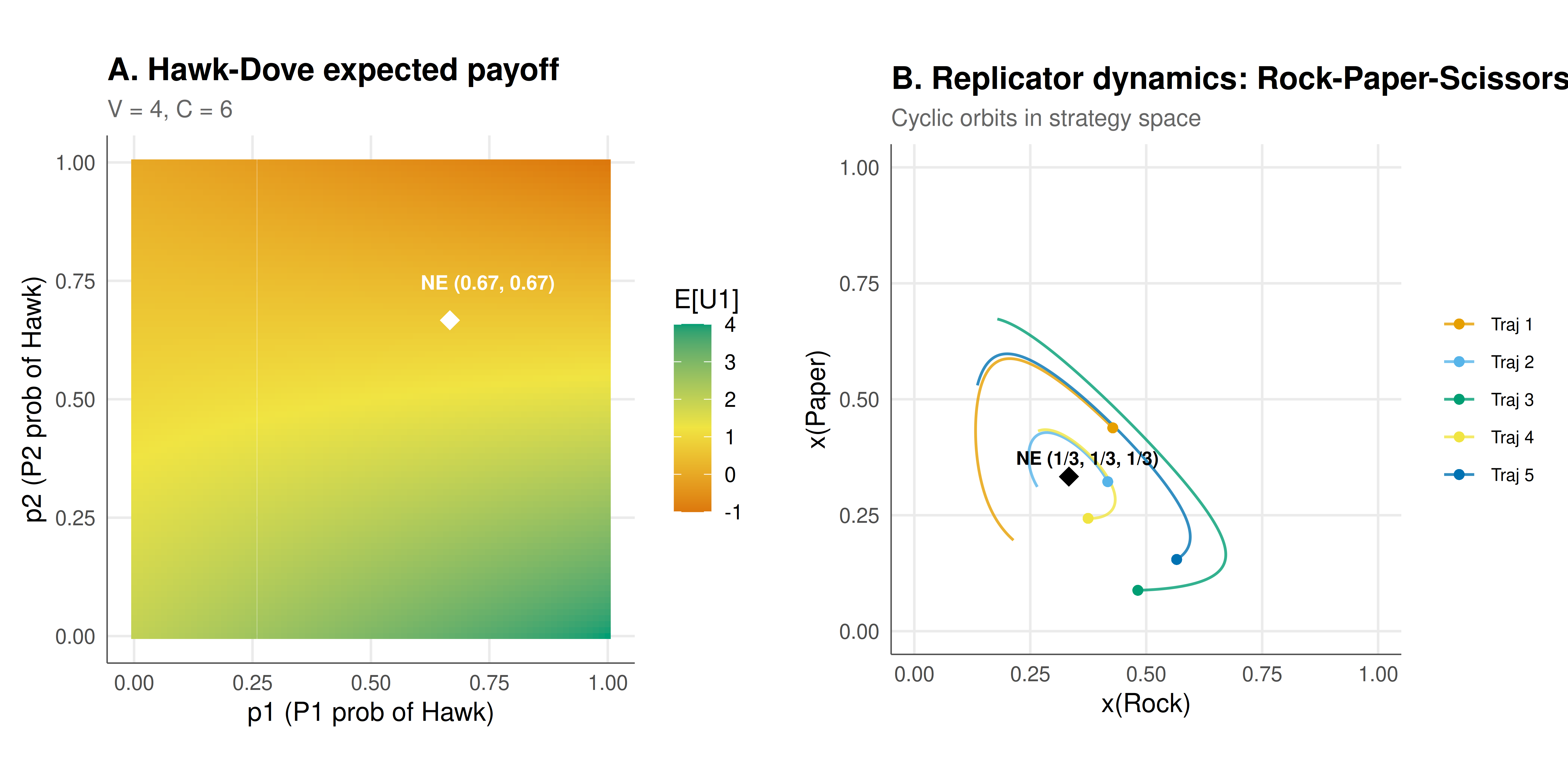
The static figure displays the Hawk-Dove expected payoff surface as a heatmap with the Nash equilibrium marked, alongside the replicator dynamics trajectories for Rock-Paper-Scissors.
```{r}
#| label: fig-dashboard-static
#| fig-cap: "Figure 1. Left: Player 1 expected payoff in the Hawk-Dove game (V=4, C=6) as a function of both players' mixing probabilities p1 (Hawk) and p2 (Hawk). The diamond marks the symmetric mixed Nash equilibrium at p* = V/C = 2/3. Right: Replicator dynamics trajectories for Rock-Paper-Scissors from 5 random initial conditions, showing cyclic orbits around the interior equilibrium (1/3, 1/3, 1/3)."
#| dev: [png, pdf]
#| fig-width: 10
#| fig-height: 5
#| dpi: 300
# Panel A: Hawk-Dove payoff heatmap
p_hd_heat <- ggplot(hd_grid, aes(x = p1, y = p2, fill = U1)) +
  geom_tile() +
  scale_fill_gradient2(
    low = okabe_ito[6], mid = okabe_ito[4], high = okabe_ito[3],
    midpoint = mean(hd_grid$U1),
    name = "E[U1]"
  ) +
  geom_point(aes(x = p_star, y = p_star), colour = "white",
             size = 4, shape = 18, inherit.aes = FALSE) +
  annotate("text", x = p_star + 0.08, y = p_star + 0.08,
           label = paste0("NE (", round(p_star, 2), ", ", round(p_star, 2), ")"),
           colour = "white", size = 3.2, fontface = "bold") +
  coord_fixed() +
  labs(
    title = "A. Hawk-Dove expected payoff",
    subtitle = paste0("V = ", V, ", C = ", C),
    x = "p1 (P1 prob of Hawk)",
    y = "p2 (P2 prob of Hawk)"
  ) +
  theme_publication() +
  theme(legend.position = "right")

# Panel B: RPS trajectories (projected to 2D: Rock vs Paper, Scissors implicit)
rps_2d <- bind_rows(traj_data) %>%
  mutate(text = paste0("Trajectory: ", trajectory,
                       "\nt = ", time,
                       "\nRock: ", round(Rock, 3),
                       "\nPaper: ", round(Paper, 3),
                       "\nScissors: ", round(Scissors, 3)))

p_rps <- ggplot(rps_2d, aes(x = Rock, y = Paper,
                             colour = trajectory, group = trajectory)) +
  geom_path(linewidth = 0.6, alpha = 0.8) +
  geom_point(data = rps_2d %>% filter(time == 0),
             shape = 16, size = 2) +
  geom_point(aes(x = 1/3, y = 1/3), colour = "black",
             size = 4, shape = 18, inherit.aes = FALSE) +
  annotate("text", x = 1/3 + 0.04, y = 1/3 + 0.04,
           label = "NE (1/3, 1/3, 1/3)", size = 3, fontface = "bold") +
  scale_colour_manual(values = okabe_ito[1:5]) +
  coord_fixed(xlim = c(0, 1), ylim = c(0, 1)) +
  labs(
    title = "B. Replicator dynamics: Rock-Paper-Scissors",
    subtitle = "Cyclic orbits in strategy space",
    x = "x(Rock)",
    y = "x(Paper)",
    colour = NULL
  ) +
  theme_publication() +
  theme(legend.position = "right", legend.text = element_text(size = 8))

gridExtra::grid.arrange(p_hd_heat, p_rps, ncol = 2)
```
## Interactive figure
This interactive figure shows the 3D expected-payoff surface for Player 1 in the Battle of the Sexes. Rotate, zoom, and hover to explore how Player 1's payoff varies across the full mixed-strategy space. The Nash equilibria are marked as red spheres.
```{r}
#| label: fig-dashboard-interactive
# 3D surface for Battle of the Sexes
U1_matrix <- matrix(bos_surface$U1, nrow = length(p_seq), ncol = length(q_seq))

fig_3d <- plot_ly() %>%
  add_surface(
    x = q_seq, y = p_seq, z = U1_matrix,
    colorscale = list(c(0, okabe_ito[5]), c(0.5, okabe_ito[4]), c(1, okabe_ito[1])),
    opacity = 0.85,
    hovertemplate = paste0(
      "q (P2 prob Opera): %{x:.3f}<br>",
      "p (P1 prob Opera): %{y:.3f}<br>",
      "E[U1]: %{z:.3f}<extra></extra>"
    ),
    showscale = TRUE,
    colorbar = list(title = "E[U1]")
  ) %>%
  add_trace(
    data = bos_ne,
    x = ~q, y = ~p, z = ~U1,
    type = "scatter3d", mode = "markers+text",
    marker = list(size = 8, color = okabe_ito[6], symbol = "circle"),
    text = ~label,
    textposition = "top center",
    textfont = list(size = 10, color = okabe_ito[6]),
    hovertemplate = paste0(
      "%{text}<br>",
      "p = %{y:.2f}, q = %{x:.2f}<br>",
      "E[U1] = %{z:.3f}<extra></extra>"
    ),
    showlegend = FALSE
  ) %>%
  layout(
    title = list(text = "Battle of the Sexes: Player 1 expected payoff surface"),
    scene = list(
      xaxis = list(title = "q (P2 prob Opera)"),
      yaxis = list(title = "p (P1 prob Opera)"),
      zaxis = list(title = "E[U1]"),
      camera = list(eye = list(x = 1.5, y = -1.5, z = 1.2))
    )
  ) %>%
  config(displaylogo = FALSE)

fig_3d
```
## Interpretation
The four dashboard components demonstrate how interactivity transforms the communication of game-theoretic concepts. The interactive payoff matrix makes the logic of best responses immediately visible: hovering over each cell reveals not only the numerical payoffs but also whether that outcome is a best response for either player, and whether it is a Nash equilibrium. In the Prisoner's Dilemma, the viewer can verify that (Defect, Defect) is the unique Nash equilibrium by inspecting the best-response annotations on each cell, even without prior knowledge of the formal definition.
The animated replicator dynamics visualisation for Rock-Paper-Scissors reveals the characteristic cyclic orbits that distinguish this game from games with asymptotically stable equilibria. By scrubbing through time, the viewer can observe how population shares oscillate around the interior equilibrium at $(1/3, 1/3, 1/3)$ without ever converging to it. Different initial conditions produce orbits of different amplitudes but the same qualitative character --- a signature of the conservative nature of the RPS dynamics (the dynamics preserve a Lyapunov function, so orbits are closed curves in the continuous-time limit) [@maynard_smith_1982].
The Hawk-Dove heatmap shows the full expected-payoff landscape, making it visually clear that the mixed Nash equilibrium at $p^* = V/C$ is a saddle-like point where neither player can unilaterally improve. The 3D surface for the Battle of the Sexes is perhaps the most pedagogically powerful: rotating the surface reveals that the two pure Nash equilibria sit at the corners (peaks for one player, valleys for the other), while the mixed Nash equilibrium lies at an intermediate point that is Pareto-dominated by both pure equilibria. This geometric insight --- that the mixed equilibrium is "worse" for both players than either pure equilibrium --- is difficult to communicate through equations alone but becomes visually obvious in 3D.
From a technical standpoint, the key `plotly` features demonstrated are `hovertemplate` for rich tooltips, `animation_frame` and `animation_opts` for temporal animations, `highlight()` for linked brushing, and `add_surface()` for 3D visualisation. These features, combined with the `ggplotly()` bridge for leveraging `ggplot2`'s grammar of graphics, provide a comprehensive toolkit for interactive game theory communication.
## Extensions & related tutorials
The interactive techniques demonstrated here can be applied to any game theory visualisation. Combine them with the site's ggplot theme system for consistent, publication-ready styling across static and interactive outputs.
- [Publication-ready ggplot theme](../../visualization-and-communication/publication-ready-ggplot-theme/) --- the custom theme system used throughout this site, providing the foundation for the static panels shown here
- [Nash's existence proof](../../history-of-gt-mathematics/nash-equilibrium-original-proof/) --- visualising best-response correspondences and fixed points, which benefit directly from the interactive techniques shown here
- [Eigenvalue methods for repeated games](../../linear-algebra-matrix/eigenvalue-methods-repeated-games/) --- convergence dynamics that can be animated using the techniques from this tutorial
- [Power-law networks and strategic behaviour](../../network-science/power-law-networks-strategic/) --- network visualisations that benefit from interactive hover and zoom
## References
::: {#refs}
:::