---
title: "Combinatorial Auctions — Bidding on Bundles of Items"
description: "Implement the winner determination problem for combinatorial auctions using integer programming with lpSolve, model a spectrum auction with complementarities, compare VCG and first-price payment rules, and demonstrate the exposure problem in R."
author: "Raban Heller"
date: 2026-05-08
date-modified: 2026-05-08
categories:
- mechanism-design
- combinatorial-auctions
- integer-programming
keywords: ["combinatorial auction", "winner determination", "VCG", "integer programming", "exposure problem"]
labels: ["auction-theory", "mechanism-design"]
tier: 1
bibliography: ../../../references.bib
vgwort: "TODO_VGWORT_mechanism-design_combinatorial-auctions"
image: thumbnail.png
image-alt: "Heatmap of bidder valuations across bundles of spectrum licences showing complementarities and the optimal allocation"
citation:
type: webpage
url: https://r-heller.github.io/equilibria/tutorials/mechanism-design/combinatorial-auctions/
license: "CC BY-SA 4.0"
draft: false
has_static_fig: true
has_interactive_fig: true
has_shiny_app: false
---
```{r}
#| label: setup
#| include: false
library(ggplot2)
library(dplyr)
library(tidyr)
library(plotly)
okabe_ito <- c("#E69F00", "#56B4E9", "#009E73", "#F0E442",
"#0072B2", "#D55E00", "#CC79A7", "#999999")
theme_publication <- function(base_size = 12) {
theme_minimal(base_size = base_size) +
theme(plot.title = element_text(size = base_size * 1.2, face = "bold"),
plot.subtitle = element_text(size = base_size * 0.9, color = "grey40"),
axis.line = element_line(color = "grey30", linewidth = 0.3),
panel.grid.minor = element_blank(), legend.position = "bottom",
plot.margin = margin(10, 10, 10, 10))
}
```
## Introduction & motivation
In many real-world allocation problems, the value of a set of items depends not just on the individual items but on which combinations are acquired together. A telecommunications company bidding for radio spectrum licences values a contiguous block of frequencies far more than scattered individual licences, because contiguous spectrum enables higher bandwidth and better service quality. An airline bidding for airport landing slots values a pair of slots (departure and arrival) much more than either slot alone, because a single slot without its complement is nearly useless. An advertiser buying ad placements values a combination of slots across different media more than the sum of individual placements, because cross-platform campaigns have synergistic reach effects. In all these cases, items are **complementary**: the value of the bundle exceeds the sum of the individual item values.
**Combinatorial auctions** address this by allowing bidders to submit bids on arbitrary bundles (combinations) of items, rather than forcing them to bid on items one at a time. This seemingly simple extension -- from single-item to bundle bidding -- has profound consequences for both the computational complexity and the economic properties of the auction. The central computational challenge is the **winner determination problem (WDP)**: given a set of bids on various bundles, find the allocation of items to bidders that maximises total revenue (or social welfare), subject to the constraint that each item is allocated to at most one bidder. This problem is NP-hard in general, meaning that no polynomial-time algorithm is known and the computational difficulty grows exponentially with the number of items and bids. In practice, the WDP is formulated as an integer linear program and solved using branch-and-bound or cutting-plane methods.
The economic design of combinatorial auctions raises equally challenging questions. The **Vickrey-Clarke-Groves (VCG) mechanism** extends the truthful Vickrey second-price auction to the combinatorial setting: each winning bidder pays the externality they impose on others, which equals the total welfare of the other bidders in the optimal allocation without the given bidder minus the total welfare of the other bidders in the actual optimal allocation. Under VCG pricing, truthful bidding is a dominant strategy -- each bidder maximises their payoff by reporting their true valuations -- but VCG payments can be very low (sometimes zero), and the mechanism requires solving the WDP multiple times (once for the full allocation and once for each winning bidder excluded). **First-price payment rules**, where each winner pays their bid, are simpler but destroy the incentive for truthful bidding, leading to strategic bid shading.
Perhaps the most practically important concept in combinatorial auction design is the **exposure problem**, which arises when bidders cannot bid on bundles and must instead bid on individual items in separate simultaneous auctions. A bidder who needs a specific combination of items faces a dilemma: they might win some items in the bundle but not others, leaving them "exposed" to paying for items that are worthless without their complements. The exposure problem was a primary motivation for the design of combinatorial auction formats and played a central role in the debates surrounding the FCC spectrum auctions in the United States in the 1990s and 2000s.
In this tutorial, we model a spectrum auction with three bidders competing for four licences. We formulate and solve the winner determination problem using `lpSolve`, implement both VCG and first-price payment rules, and demonstrate the exposure problem through simulation. The example is small enough for exact computation but rich enough to illustrate all the key phenomena.
## Mathematical formulation
**Items.** Let $M = \{1, 2, \ldots, m\}$ be a set of $m$ items. A **bundle** is a subset $S \subseteq M$.
**Bidders and valuations.** Bidder $i \in N = \{1, \ldots, n\}$ has a valuation function $v_i: 2^M \to \mathbb{R}_{\geq 0}$ with $v_i(\emptyset) = 0$.
**Complementarities**: Items $j, k$ are complements for bidder $i$ if $v_i(\{j,k\}) > v_i(\{j\}) + v_i(\{k\})$.
**Substitutes**: Items $j, k$ are substitutes if $v_i(\{j,k\}) < v_i(\{j\}) + v_i(\{k\})$.
**Winner Determination Problem (WDP).** Given bids $b_{ij}$ for bidder $i$ on bundle $S_j$:
$$
\max \sum_{i,j} b_{ij} \cdot x_{ij}
$$
subject to:
$$
\sum_{i,j: k \in S_j} x_{ij} \leq 1 \quad \forall\, k \in M \qquad \text{(each item allocated at most once)}
$$
$$
\sum_{j} x_{ij} \leq 1 \quad \forall\, i \in N \qquad \text{(each bidder wins at most one bundle)}
$$
$$
x_{ij} \in \{0, 1\}
$$
**VCG payments.** Let $W^*$ be the optimal social welfare. Let $W^*_{-i}$ be the optimal welfare when bidder $i$ is excluded. Bidder $i$'s VCG payment is:
$$
p_i^{VCG} = W^*_{-i} - \sum_{j \neq i} v_j(S_j^*)
$$
where $S_j^*$ is the bundle allocated to bidder $j$ in the optimal allocation.
## R implementation
```{r}
#| label: combinatorial-auction
set.seed(42)

# --- Spectrum auction: 3 bidders, 4 licences ---
items <- c("A", "B", "C", "D")
n_items <- length(items)
bidders <- c("Telecom1", "Telecom2", "Telecom3")
n_bidders <- length(bidders)

# Generate all non-empty subsets (bundles)
all_bundles <- list()
bundle_labels <- character()
for (k in 1:n_items) {
  combos <- combn(items, k, simplify = FALSE)
  for (combo in combos) {
    all_bundles <- c(all_bundles, list(combo))
    bundle_labels <- c(bundle_labels, paste(combo, collapse = "+"))
  }
}
n_bundles <- length(all_bundles)

# Valuation functions with complementarities
# Telecom1: values contiguous blocks {A,B} and {A,B,C}
# Telecom2: values {C,D} and {B,C,D}
# Telecom3: moderate values, wants any 2 adjacent licences
single_values <- matrix(c(
  # A    B    C    D
   30,  25,  10,   5,  # Telecom1
    5,  10,  30,  25,  # Telecom2
   15,  20,  20,  15   # Telecom3
), nrow = 3, byrow = TRUE, dimnames = list(bidders, items))

# Compute bundle values with complementarity
compute_bundle_value <- function(bidder_idx, bundle) {
  base_val <- sum(single_values[bidder_idx, bundle])

  # Complementarity bonus for contiguous blocks
  if (bidder_idx == 1) {
    if (all(c("A", "B") %in% bundle)) base_val <- base_val + 25
    if (all(c("A", "B", "C") %in% bundle)) base_val <- base_val + 20
  } else if (bidder_idx == 2) {
    if (all(c("C", "D") %in% bundle)) base_val <- base_val + 25
    if (all(c("B", "C", "D") %in% bundle)) base_val <- base_val + 20
  } else {
    if (length(bundle) >= 2) base_val <- base_val + 10
  }
  return(base_val)
}

# Build valuation matrix: bidders x bundles
val_matrix <- matrix(0, n_bidders, n_bundles,
                      dimnames = list(bidders, bundle_labels))
for (i in 1:n_bidders) {
  for (j in 1:n_bundles) {
    val_matrix[i, j] <- compute_bundle_value(i, all_bundles[[j]])
  }
}

cat("=== Valuation Matrix (selected bundles) ===\n")
show_bundles <- c("A", "B", "C", "D", "A+B", "C+D", "A+B+C", "B+C+D", "A+B+C+D")
for (bl in show_bundles) {
  if (bl %in% bundle_labels) {
    idx <- which(bundle_labels == bl)
    cat(sprintf("  %-8s: T1=%3d  T2=%3d  T3=%3d\n", bl,
                val_matrix[1, idx], val_matrix[2, idx], val_matrix[3, idx]))
  }
}
# --- Winner Determination Problem using lpSolve ---
# Decision variables: x[i,j] = 1 if bidder i wins bundle j
n_vars <- n_bidders * n_bundles

# Objective: maximise total value (assume truthful bidding)
obj <- as.vector(t(val_matrix))

# Constraints
# 1. Each item allocated at most once
item_constraints <- matrix(0, n_items, n_vars)
for (k in 1:n_items) {
  for (i in 1:n_bidders) {
    for (j in 1:n_bundles) {
      if (items[k] %in% all_bundles[[j]]) {
        col_idx <- (i - 1) * n_bundles + j
        item_constraints[k, col_idx] <- 1
      }
    }
  }
}

# 2. Each bidder wins at most one bundle
bidder_constraints <- matrix(0, n_bidders, n_vars)
for (i in 1:n_bidders) {
  cols <- ((i - 1) * n_bundles + 1):(i * n_bundles)
  bidder_constraints[i, cols] <- 1
}

constraint_matrix <- rbind(item_constraints, bidder_constraints)
constraint_dir <- rep("<=", n_items + n_bidders)
constraint_rhs <- c(rep(1, n_items), rep(1, n_bidders))

# Solve
result <- lpSolve::lp("max", obj, constraint_matrix, constraint_dir, constraint_rhs,
                        all.bin = TRUE)

cat(sprintf("\n=== Optimal Allocation (Social Welfare = %d) ===\n", result$objval))
# Decode solution
allocation <- list()
for (i in 1:n_bidders) {
  cols <- ((i - 1) * n_bundles + 1):(i * n_bundles)
  won <- which(result$solution[cols] == 1)
  if (length(won) > 0) {
    allocation[[bidders[i]]] <- list(
      bundle = bundle_labels[won],
      value = val_matrix[i, won]
    )
    cat(sprintf("  %s wins bundle {%s}, value = %d\n",
                bidders[i], bundle_labels[won], val_matrix[i, won]))
  } else {
    allocation[[bidders[i]]] <- list(bundle = "none", value = 0)
    cat(sprintf("  %s wins nothing\n", bidders[i]))
  }
}
# --- VCG Payments ---
cat("\n=== VCG Payments ===\n")
total_welfare <- result$objval

vcg_payments <- numeric(n_bidders)
names(vcg_payments) <- bidders

for (i in 1:n_bidders) {
  # Welfare of others in current allocation
  others_welfare_current <- sum(sapply(setdiff(1:n_bidders, i), function(j) {
    cols <- ((j - 1) * n_bundles + 1):(j * n_bundles)
    won <- which(result$solution[cols] == 1)
    if (length(won) > 0) val_matrix[j, won] else 0
  }))

  # Optimal welfare without bidder i
  obj_minus_i <- obj
  cols_i <- ((i - 1) * n_bundles + 1):(i * n_bundles)
  obj_minus_i[cols_i] <- 0

  result_minus_i <- lpSolve::lp("max", obj_minus_i, constraint_matrix,
                                  constraint_dir, constraint_rhs, all.bin = TRUE)
  others_welfare_without <- result_minus_i$objval

  vcg_payments[i] <- others_welfare_without - others_welfare_current

  cat(sprintf("  %s: VCG payment = %d (externality imposed on others)\n",
              bidders[i], vcg_payments[i]))
}
cat(sprintf("\n Total VCG revenue: %d\n", sum(vcg_payments)))
cat(sprintf(" Total welfare: %d\n", total_welfare))
# --- First-price payments (pay your bid) ---
cat("\n=== First-Price vs VCG ===\n")
for (i in 1:n_bidders) {
  fp_payment <- allocation[[bidders[i]]]$value
  cat(sprintf("  %s: First-price = %d, VCG = %d, Savings = %d\n",
              bidders[i], fp_payment, vcg_payments[i],
              fp_payment - vcg_payments[i]))
}
# --- Exposure Problem Simulation ---
cat("\n=== Exposure Problem ===\n")
cat("Simulating item-by-item auctions (no bundle bidding)...\n")
# Each item sold in separate second-price auction
# Telecom1 bids for A and B (wants {A,B} bundle)
# Telecom2 bids for C and D (wants {C,D} bundle)
# Telecom3 bids competitively on all items

n_exposure_sims <- 1000
exposure_results <- tibble(
  sim = 1:n_exposure_sims,
  t1_items_won = integer(n_exposure_sims),
  t1_value = numeric(n_exposure_sims),
  t1_payment = numeric(n_exposure_sims),
  t1_profit = numeric(n_exposure_sims)
)

for (s in 1:n_exposure_sims) {
  # Add noise to bids (strategic uncertainty)
  noise <- matrix(rnorm(n_bidders * n_items, 0, 5), n_bidders, n_items)
  bids <- pmax(0, single_values + noise)

  t1_won <- character()
  t1_pay <- 0

  for (k in 1:n_items) {
    # Second-price auction for item k
    item_bids <- bids[, k]
    winner <- which.max(item_bids)
    price <- sort(item_bids, decreasing = TRUE)[2]  # second-highest bid

    if (winner == 1) {
      t1_won <- c(t1_won, items[k])
      t1_pay <- t1_pay + price
    }
  }

  t1_bundle_val <- if (length(t1_won) > 0) compute_bundle_value(1, t1_won) else 0
  exposure_results$t1_items_won[s] <- length(t1_won)
  exposure_results$t1_value[s] <- t1_bundle_val
  exposure_results$t1_payment[s] <- t1_pay
  exposure_results$t1_profit[s] <- t1_bundle_val - t1_pay
}
cat(sprintf("  Telecom1 wins complete {A,B} bundle: %.1f%% of the time\n",
            100 * mean(exposure_results$t1_items_won >= 2)))
cat(sprintf("  Telecom1 wins only 1 item (exposed!): %.1f%% of the time\n",
            100 * mean(exposure_results$t1_items_won == 1)))
cat(sprintf(" Telecom1 average profit: %.1f\n", mean(exposure_results$t1_profit)))
cat(sprintf("  Telecom1 negative profit (loss): %.1f%% of simulations\n",
            100 * mean(exposure_results$t1_profit < 0)))
```
## Static publication-ready figure
```{r}
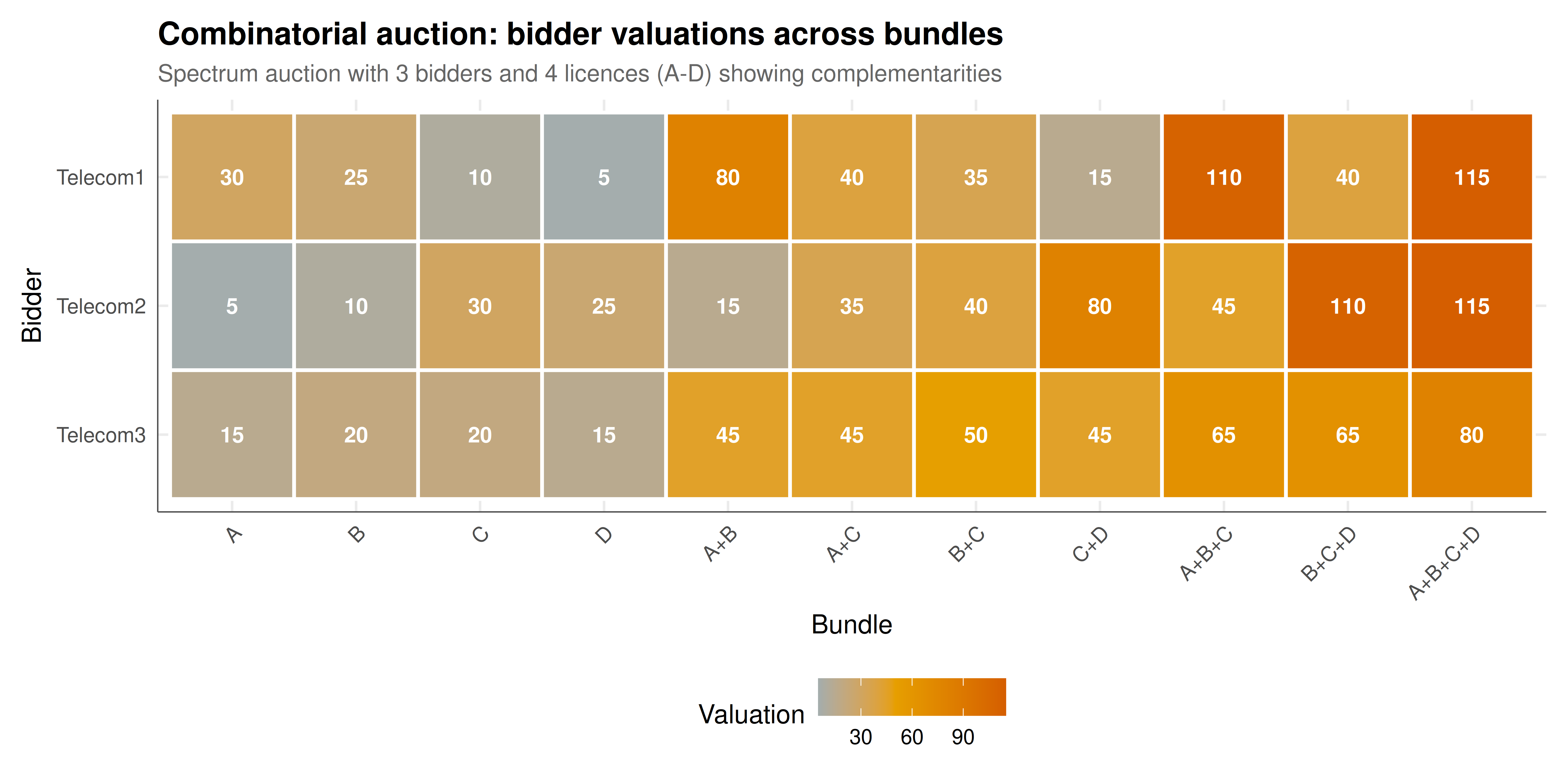
#| label: fig-auction-valuations
#| fig-cap: "Figure 1. Bundle valuations for three telecom bidders in a spectrum auction with four licences (A-D). Super-additive valuations (complementarities) are visible where bundle values exceed the sum of individual item values. Telecom1 values the {A,B} bundle at 80 (vs 30+25=55 individually), showing strong complementarity for contiguous spectrum. The optimal allocation assigns {A,B} to Telecom1 and {C,D} to Telecom2. Okabe-Ito palette."
#| dev: [png, pdf]
#| fig-width: 10
#| fig-height: 5
#| dpi: 300
# Create heatmap of valuations for key bundles
key_bundles <- c("A", "B", "C", "D", "A+B", "A+C", "B+C", "C+D",
                  "A+B+C", "B+C+D", "A+B+C+D")
key_idx <- which(bundle_labels %in% key_bundles)

heat_df <- tibble(
  bidder = rep(bidders, each = length(key_bundles)),
  bundle = rep(key_bundles, n_bidders),
  value = as.vector(t(val_matrix[, key_idx]))
) |>
  mutate(bundle = factor(bundle, levels = key_bundles),
         bidder = factor(bidder, levels = rev(bidders)))

# Mark complementarity
heat_df <- heat_df |>
  mutate(
    sum_parts = case_when(
      bundle == "A+B" & bidder == "Telecom1" ~ 55,
      bundle == "C+D" & bidder == "Telecom2" ~ 55,
      bundle == "A+B" & bidder == "Telecom2" ~ 15,
      bundle == "C+D" & bidder == "Telecom1" ~ 15,
      TRUE ~ NA_real_
    ),
    complementarity = ifelse(!is.na(sum_parts), value - sum_parts, NA_real_),
    label = as.character(value)
  )

p_heat <- ggplot(heat_df, aes(x = bundle, y = bidder, fill = value)) +
  geom_tile(color = "white", linewidth = 0.8) +
  geom_text(aes(label = label), size = 3.5, color = "white", fontface = "bold") +
  scale_fill_gradient2(low = okabe_ito[2], mid = okabe_ito[1], high = okabe_ito[6],
                        midpoint = 50, name = "Valuation") +
  labs(title = "Combinatorial auction: bidder valuations across bundles",
       subtitle = "Spectrum auction with 3 bidders and 4 licences (A-D) showing complementarities",
       x = "Bundle", y = "Bidder") +
  theme_publication() +
  theme(axis.text.x = element_text(angle = 45, hjust = 1))

p_heat
```
## Interactive figure
```{r}
#| label: fig-exposure-interactive
# Show exposure problem distribution
exposure_plot <- exposure_results |>
  mutate(
    outcome = case_when(
      t1_items_won == 0 ~ "Won nothing",
      t1_items_won == 1 ~ "Exposed (1 item)",
      t1_items_won >= 2 ~ "Won 2+ items"
    ),
    outcome = factor(outcome, levels = c("Won nothing", "Exposed (1 item)", "Won 2+ items")),
    text = paste0("Sim: ", sim,
                  "\nItems won: ", t1_items_won,
                  "\nBundle value: ", round(t1_value, 0),
                  "\nPayment: ", round(t1_payment, 0),
                  "\nProfit: ", round(t1_profit, 0))
  )

p_exposure <- ggplot(exposure_plot, aes(x = t1_payment, y = t1_profit,
                                          color = outcome, text = text)) +
  geom_point(alpha = 0.5, size = 1.5) +
  geom_hline(yintercept = 0, linetype = "dashed", color = "grey50") +
  scale_color_manual(values = c("Won nothing" = okabe_ito[8],
                                 "Exposed (1 item)" = okabe_ito[6],
                                 "Won 2+ items" = okabe_ito[3]),
                      name = "Outcome") +
  labs(title = "Exposure problem: Telecom1's profit in item-by-item auctions",
       subtitle = "Without bundle bidding, winning partial bundles leads to losses",
       x = "Total payment", y = "Profit (value - payment)") +
  theme_publication()

ggplotly(p_exposure, tooltip = "text") |>
  config(displaylogo = FALSE,
         modeBarButtonsToRemove = c("select2d", "lasso2d"))
```
## Interpretation
The results of our spectrum auction model illustrate the core economic insights of combinatorial auction theory. The optimal allocation, found by solving the winner determination problem as an integer program, assigns the {A,B} bundle to Telecom1 and the {C,D} bundle to Telecom2, reflecting their complementary valuations for contiguous spectrum blocks. This allocation achieves a social welfare substantially higher than any allocation that splits contiguous blocks, demonstrating why combinatorial auctions are worth the additional complexity: by allowing bidders to express complementarities directly, the mechanism can find allocations that would be impossible to discover through separate item-by-item auctions.
The VCG payment comparison reveals one of the most important features and one of the most important criticisms of the VCG mechanism. Each bidder pays not their bid but the externality they impose on others -- the difference between the optimal welfare achievable by others without the bidder and the welfare actually received by others. This makes truthful bidding a dominant strategy: no bidder can improve their outcome by misreporting their valuations. However, the VCG payments are significantly lower than the first-price payments, meaning that the auctioneer (government, in the spectrum case) collects less revenue under VCG. This revenue gap is a well-known drawback of VCG and has led to its rare use in practice -- the FCC's spectrum auctions, for example, use ascending clock auctions rather than sealed-bid VCG formats. The choice between revenue maximisation and incentive compatibility is a fundamental tension in mechanism design, and there is no general mechanism that achieves both simultaneously.
The exposure problem simulation provides the most practically compelling argument for combinatorial auctions. When Telecom1 bids in separate item-by-item second-price auctions, they face a severe risk: they may win item A but not item B (or vice versa), leaving them with a single licence worth far less than the complementary pair. In our simulation, this "exposed" outcome occurs in a significant fraction of cases, and it frequently leads to negative profits -- Telecom1 pays for an item that is nearly worthless without its complement. This is not a failure of bidding strategy; it is a structural problem with the auction format. No matter how Telecom1 adjusts their bids in the separate auctions, they cannot eliminate the exposure risk without either bidding so cautiously that they rarely win anything (the demand reduction strategy) or bidding aggressively and accepting the risk of costly incomplete bundles. Combinatorial auctions eliminate this problem by construction, since bidders can condition their payments on receiving the complete bundle.
The computational complexity dimension deserves emphasis. Our example with 4 items has $2^4 - 1 = 15$ non-empty bundles, making exhaustive enumeration trivial. But real spectrum auctions involve dozens or hundreds of licences, yielding an astronomical number of possible bundles. The winner determination problem is NP-hard, and practical implementations rely on sophisticated integer programming solvers (such as CPLEX or Gurobi) with problem-specific cuts and heuristics. The computational challenge has inspired a productive dialogue between computer scientists and economists, leading to the development of computationally tractable auction formats such as the combinatorial clock auction (CCA) used in recent European spectrum sales. These formats sacrifice some theoretical optimality for computational tractability, accepting approximate rather than exact solutions to the winner determination problem. The interplay between incentive compatibility, computational feasibility, and revenue properties remains one of the most active research areas in mechanism design.
## Extensions & related tutorials
- [Vickrey second-price auction](../vickrey-second-price-auction/) -- the single-item auction that VCG generalises.
- [VCG mechanism](../vcg-mechanism/) -- the general Vickrey-Clarke-Groves mechanism for public goods and multi-item allocation.
- [Mechanism design introduction](../mechanism-design-intro/) -- foundational concepts of incentive-compatible mechanism design.
- [Deferred acceptance algorithm](../deferred-acceptance/) -- matching mechanisms for two-sided markets.
- [Fair division and cake-cutting](../../ethics-and-game-theory/fair-division-cake-cutting/) -- alternative approaches to allocating heterogeneous goods.
## References
::: {#refs}
:::