---
title: "Multi-agent reinforcement learning in matrix games"
description: "Implement independent Q-learning agents that learn to play 2x2 matrix games, analyse convergence behaviour across game classes, and investigate when learning dynamics converge (or fail to converge) to Nash equilibria."
author: "Raban Heller"
date: 2026-05-08
categories:
- ml-and-gt
- reinforcement-learning
- multi-agent
keywords: ["Q-learning", "multi-agent reinforcement learning", "MARL", "Nash equilibrium", "convergence", "matrix games", "independent learners", "R"]
labels: ["machine-learning", "multi-agent-systems"]
tier: 1
bibliography: ../../../references.bib
vgwort: "TODO_VGWORT_ml-and-gt_multi-agent-reinforcement-learning"
image: thumbnail.png
image-alt: "Time series showing Q-learning agents converging to Nash equilibrium mixing probabilities in a matrix game"
citation:
type: webpage
url: https://r-heller.github.io/equilibria/tutorials/ml-and-gt/multi-agent-reinforcement-learning/
license: "CC BY-SA 4.0"
draft: false
has_static_fig: true
has_interactive_fig: true
---
```{r}
#| label: setup
#| include: false
library(ggplot2)
library(dplyr)
library(tidyr)
library(plotly)
okabe_ito <- c("#E69F00", "#56B4E9", "#009E73", "#F0E442",
"#0072B2", "#D55E00", "#CC79A7", "#999999")
theme_publication <- function(base_size = 12) {
theme_minimal(base_size = base_size) +
theme(
plot.title = element_text(size = base_size * 1.2, face = "bold"),
plot.subtitle = element_text(size = base_size * 0.9, color = "grey40"),
axis.line = element_line(color = "grey30", linewidth = 0.3),
panel.grid.minor = element_blank(),
legend.position = "bottom",
plot.margin = margin(10, 10, 10, 10)
)
}
```
## Introduction & motivation
When multiple autonomous agents interact repeatedly in a strategic environment, each agent faces a non-stationary learning problem: the "environment" includes other agents who are simultaneously adapting their strategies. Multi-agent reinforcement learning (MARL) sits at the intersection of game theory and machine learning, asking whether independent learners can discover equilibrium behaviour through experience alone, without knowledge of the game structure or opponents' strategies. The simplest setting for this investigation is the repeated matrix game, where two Q-learning agents independently maintain value estimates for their actions and update them based on observed rewards. In games with pure-strategy Nash equilibria (like the Prisoner's Dilemma), independent Q-learners typically converge — both agents learn to play the dominant strategy. But in games requiring mixed strategies (like Matching Pennies), convergence is far from guaranteed: the non-stationarity introduced by simultaneous learning can cause cycling, divergence, or convergence to non-equilibrium behaviour. This failure of naive independent learning to find mixed Nash equilibria is one of the foundational negative results in MARL and motivates more sophisticated algorithms like Win-or-Learn-Fast (WoLF), policy hill-climbing, and opponent-modelling approaches. This tutorial implements independent Q-learning for 2x2 games in R, runs simulations across multiple game classes, and visualises the learning trajectories to build intuition about when and why convergence succeeds or fails.
## Mathematical formulation
Consider a repeated 2-player game with payoff matrices $(A, B)$. Each agent $k \in \{1, 2\}$ maintains Q-values $Q_k(a)$ for each action $a$ and selects actions using a Boltzmann (softmax) exploration policy:
$$
\pi_k(a) = \frac{\exp(Q_k(a) / \tau)}{\sum_{a'} \exp(Q_k(a') / \tau)}
$$
where $\tau > 0$ is the temperature parameter controlling exploration. After both agents select actions $(a_1, a_2)$ and receive payoffs $(r_1, r_2)$, each updates its Q-value:
$$
Q_k(a_k) \leftarrow Q_k(a_k) + \alpha \left[ r_k - Q_k(a_k) \right]
$$
where $\alpha \in (0, 1]$ is the learning rate. The **implied mixed strategy** of agent $k$ is $\pi_k$ as defined above. We say the agents **converge to a Nash equilibrium** $(\mathbf{x}^*, \mathbf{y}^*)$ if $\pi_k \to \mathbf{x}^*_k$ as the number of episodes grows.
For stationary opponents, single-agent Q-learning converges to the best response. However, when both agents learn simultaneously, the joint process $(Q_1, Q_2)$ is a coupled dynamical system with no general convergence guarantee to Nash equilibria.
## R implementation
We implement independent Q-learning agents and simulate their interaction across different 2x2 games.
```{r}
#| label: marl-implementation
# Independent Q-learning for 2x2 matrix games
run_q_learning <- function(A, B, n_episodes = 5000, alpha = 0.1,
                           tau_init = 1.0, tau_decay = 0.999,
                           seed = 42) {
  set.seed(seed)

  # Initialize Q-values
  Q1 <- c(0, 0)  # Player 1: Q(row 1), Q(row 2)
  Q2 <- c(0, 0)  # Player 2: Q(col 1), Q(col 2)

  # Storage for trajectories
  history <- tibble(
    episode = integer(),
    p1_prob_a1 = double(),
    p2_prob_a1 = double(),
    reward_1 = double(),
    reward_2 = double()
  )

  tau <- tau_init

  for (ep in seq_len(n_episodes)) {
    # Boltzmann action selection
    p1_probs <- exp(Q1 / tau) / sum(exp(Q1 / tau))
    p2_probs <- exp(Q2 / tau) / sum(exp(Q2 / tau))

    a1 <- sample(1:2, 1, prob = p1_probs)
    a2 <- sample(1:2, 1, prob = p2_probs)

    r1 <- A[a1, a2]
    r2 <- B[a1, a2]

    # Q-value updates
    Q1[a1] <- Q1[a1] + alpha * (r1 - Q1[a1])
    Q2[a2] <- Q2[a2] + alpha * (r2 - Q2[a2])

    tau <- max(tau * tau_decay, 0.01)

    if (ep %% 10 == 0) {
      p1_final <- exp(Q1 / tau) / sum(exp(Q1 / tau))
      p2_final <- exp(Q2 / tau) / sum(exp(Q2 / tau))
      history <- bind_rows(history, tibble(
        episode = ep,
        p1_prob_a1 = p1_final[1],
        p2_prob_a1 = p2_final[1],
        reward_1 = r1,
        reward_2 = r2
      ))
    }
  }
  history
}

# Define game matrices
games <- list(
  "Prisoner's Dilemma" = list(
    A = matrix(c(3, 0, 5, 1), nrow = 2, byrow = TRUE),
    B = matrix(c(3, 5, 0, 1), nrow = 2, byrow = TRUE),
    ne_p1 = 0, ne_p2 = 0  # pure NE at (D,D) = (row 2, col 2)
  ),
  "Matching Pennies" = list(
    A = matrix(c(1, -1, -1, 1), nrow = 2, byrow = TRUE),
    B = matrix(c(-1, 1, 1, -1), nrow = 2, byrow = TRUE),
    ne_p1 = 0.5, ne_p2 = 0.5
  ),
  "Battle of the Sexes" = list(
    A = matrix(c(3, 0, 0, 2), nrow = 2, byrow = TRUE),
    B = matrix(c(2, 0, 0, 3), nrow = 2, byrow = TRUE),
    ne_p1 = 0.6, ne_p2 = 0.4  # mixed NE
  )
)

# Run simulations
all_results <- bind_rows(lapply(names(games), function(gname) {
  g <- games[[gname]]
  hist <- run_q_learning(g$A, g$B, n_episodes = 10000, alpha = 0.05,
                          tau_init = 1.0, tau_decay = 0.9995)
  hist$game <- gname
  hist$ne_p1 <- g$ne_p1
  hist$ne_p2 <- g$ne_p2
  hist
}))

# Summary of final strategies
final_strats <- all_results |>
  group_by(game) |>
  slice_tail(n = 50) |>
  summarise(
    mean_p1 = mean(p1_prob_a1),
    mean_p2 = mean(p2_prob_a1),
    ne_p1 = first(ne_p1),
    ne_p2 = first(ne_p2),
    .groups = "drop"
  )

cat("=== Final learned strategies vs Nash equilibrium ===\n")
print(as.data.frame(final_strats))
```
## Static publication-ready figure
```{r}
#| label: fig-marl-trajectories-static
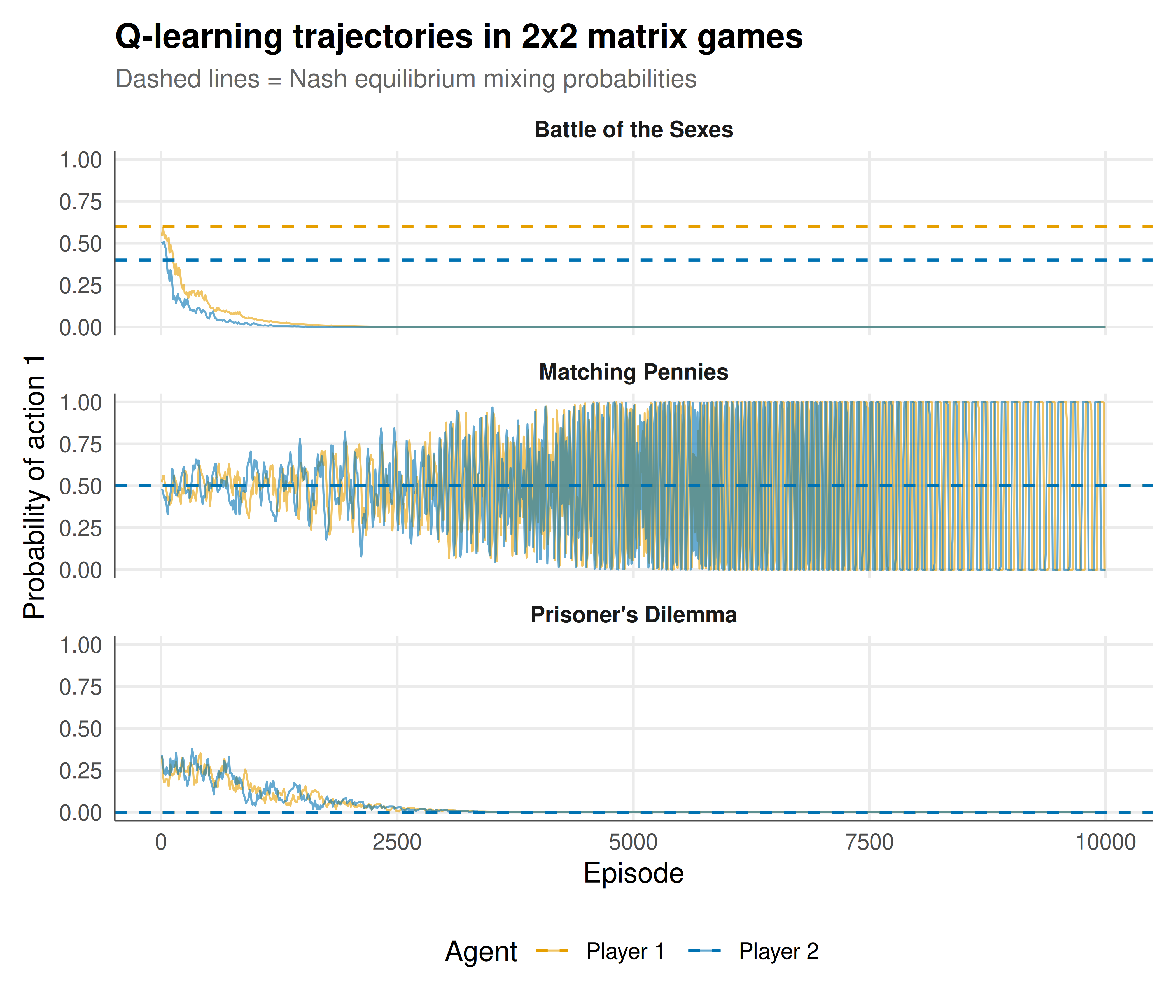
#| fig-cap: "Figure 1. Q-learning strategy trajectories across three game classes. The dashed horizontal lines mark the Nash equilibrium mixing probability. In the Prisoner's Dilemma, agents converge to the dominant strategy (defect). In Matching Pennies, agents oscillate around the mixed NE without stable convergence — the hallmark of independent learning in zero-sum games. In Battle of the Sexes, convergence depends on initial conditions and may reach a pure or mixed NE. Okabe-Ito palette."
#| dev: [png, pdf]
#| fig-width: 7
#| fig-height: 6
#| dpi: 300
results_long <- all_results |>
  pivot_longer(cols = c(p1_prob_a1, p2_prob_a1),
               names_to = "player",
               values_to = "prob_action_1") |>
  mutate(player = recode(player,
    "p1_prob_a1" = "Player 1",
    "p2_prob_a1" = "Player 2"
  ))

ne_lines <- all_results |>
  distinct(game, ne_p1, ne_p2) |>
  pivot_longer(cols = c(ne_p1, ne_p2),
               names_to = "player",
               values_to = "ne_value") |>
  mutate(player = recode(player,
    "ne_p1" = "Player 1",
    "ne_p2" = "Player 2"
  ))

p_traj <- ggplot(results_long, aes(x = episode, y = prob_action_1, color = player)) +
  geom_line(alpha = 0.6, linewidth = 0.4) +
  geom_hline(data = ne_lines, aes(yintercept = ne_value, color = player),
             linetype = "dashed", linewidth = 0.6) +
  facet_wrap(~game, ncol = 1, scales = "free_y") +
  scale_color_manual(values = c("Player 1" = okabe_ito[1],
                                  "Player 2" = okabe_ito[5]),
                      name = "Agent") +
  scale_y_continuous(limits = c(0, 1)) +
  labs(
    title = "Q-learning trajectories in 2x2 matrix games",
    subtitle = "Dashed lines = Nash equilibrium mixing probabilities",
    x = "Episode", y = "Probability of action 1"
  ) +
  theme_publication() +
  theme(strip.text = element_text(face = "bold"))

p_traj
```
## Interactive figure
```{r}
#| label: fig-marl-phase-interactive
# Phase portrait: P1 mixing prob vs P2 mixing prob over time
phase_data <- all_results |>
  mutate(text = paste0("Episode: ", episode,
                       "\nP1 prob(a1): ", round(p1_prob_a1, 3),
                       "\nP2 prob(a1): ", round(p2_prob_a1, 3)))

p_phase <- ggplot(phase_data, aes(x = p1_prob_a1, y = p2_prob_a1,
                                    color = episode, text = text)) +
  geom_path(linewidth = 0.3, alpha = 0.7) +
  geom_point(data = phase_data |> group_by(game) |> slice_head(n = 1),
             shape = 17, size = 3, color = okabe_ito[3]) +
  geom_point(data = phase_data |> group_by(game) |> slice_tail(n = 1),
             shape = 15, size = 3, color = okabe_ito[6]) +
  facet_wrap(~game, ncol = 3) +
  scale_color_gradient(low = okabe_ito[2], high = okabe_ito[5], name = "Episode") +
  coord_fixed(xlim = c(0, 1), ylim = c(0, 1)) +
  labs(
    title = "Phase portraits of Q-learning dynamics",
    subtitle = "Green triangle = start, red square = end",
    x = "Player 1: P(action 1)",
    y = "Player 2: P(action 1)"
  ) +
  theme_publication() +
  theme(strip.text = element_text(face = "bold"))

ggplotly(p_phase, tooltip = "text") |>
  config(displaylogo = FALSE,
         modeBarButtonsToRemove = c("select2d", "lasso2d"))
```
## Interpretation
The simulation results reveal the fundamental challenge of multi-agent reinforcement learning: convergence depends critically on the game structure. In the Prisoner's Dilemma, where the Nash equilibrium is in pure strategies (mutual defection), independent Q-learners converge reliably because the dominant strategy yields consistently higher rewards regardless of the opponent's evolving policy. The Q-values for defection grow steadily while those for cooperation decay, and the Boltzmann policy concentrates on the dominant action. In Matching Pennies, the situation is dramatically different. The zero-sum structure means that any predictable pattern by one agent is immediately exploited by the other, driving the first agent to change — which in turn is exploited, creating persistent oscillations. The phase portrait shows cycling behaviour rather than convergence to the mixed NE at $(0.5, 0.5)$. This is not a failure of implementation but a fundamental property of independent learning in zero-sum games: the joint Q-value dynamics form a non-convergent system. Battle of the Sexes occupies a middle ground with multiple equilibria. The learning trajectory is highly sensitive to early experiences — initial lucky coordination on one pure NE can create a self-reinforcing dynamic where both agents lock in to that equilibrium, bypassing the Pareto-inferior mixed NE entirely. This path dependence illustrates why the question "do agents converge to Nash equilibrium?" has no single answer — it depends on the game class, the learning algorithm, the exploration schedule, and even the random seed.
## Extensions & related tutorials
- [Fictitious play and belief-based learning](../../ml-and-gt/fictitious-play/) — a classical alternative to Q-learning.
- [Win-or-Learn-Fast (WoLF) dynamics](../../ml-and-gt/wolf-phc/) — gradient-based MARL with convergence guarantees.
- [Matching Pennies — pure conflict and minimax](../../classical-games/matching-pennies/) — the game theory behind the hardest case.
- [Evolutionary game dynamics](../../evolutionary-gt/replicator-dynamics/) — population-level learning as an alternative to agent-level.
- [The Prisoner's Dilemma — formal setup](../../classical-games/prisoners-dilemma-formal/) — the game where Q-learning succeeds.
## References
::: {#refs}
:::