---
title: "No-regret learning in games: from multiplicative weights to equilibrium"
description: "Implement the Multiplicative Weights Update algorithm and show that when all players use no-regret learning, the time-averaged strategy profile converges to a coarse correlated equilibrium."
author: "Raban Heller"
date: 2026-05-08
date-modified: 2026-05-08
categories:
- ml-and-gt
- no-regret-learning
- online-learning
keywords: ["no-regret learning", "multiplicative weights", "coarse correlated equilibrium", "online learning", "convergence", "R"]
labels: ["machine-learning", "online-learning"]
tier: 1
bibliography: ../../../references.bib
vgwort: "TODO_VGWORT_ML-AND-GT_NO-REGRET-LEARNING-GAMES"
image: thumbnail.png
image-alt: "Time series showing convergence of empirical strategy frequencies to equilibrium in Rock-Paper-Scissors under multiplicative weights update"
citation:
type: webpage
url: https://r-heller.github.io/equilibria/tutorials/ml-and-gt/no-regret-learning-games/
license: "CC BY-SA 4.0"
draft: false
has_static_fig: true
has_interactive_fig: true
has_shiny_app: false
---
```{r}
#| label: setup
#| include: false
library(ggplot2)
library(dplyr)
library(tidyr)
library(plotly)
okabe_ito <- c("#E69F00", "#56B4E9", "#009E73", "#F0E442",
"#0072B2", "#D55E00", "#CC79A7", "#999999")
theme_publication <- function(base_size = 12) {
theme_minimal(base_size = base_size) +
theme(plot.title = element_text(size = base_size * 1.2, face = "bold"),
plot.subtitle = element_text(size = base_size * 0.9, color = "grey40"),
axis.line = element_line(color = "grey30", linewidth = 0.3),
panel.grid.minor = element_blank(), legend.position = "bottom",
plot.margin = margin(10, 10, 10, 10))
}
```
## Introduction & motivation
One of the deepest questions in game theory is how players arrive at equilibrium. Classical equilibrium concepts --- Nash equilibrium, correlated equilibrium, and their refinements --- describe stable states from which no player has an incentive to deviate, but they say little about the dynamic process by which rational agents might discover these states. The theory of **no-regret learning** provides a powerful answer: if every player in a game independently runs a learning algorithm that guarantees low **regret** (the difference between their actual payoff and the payoff they would have obtained by playing the best fixed strategy in hindsight), then the resulting time-averaged play converges to a well-defined equilibrium concept. Specifically, the empirical distribution of play converges to the set of **coarse correlated equilibria**, a relaxation of Nash equilibrium that is both theoretically attractive and computationally tractable [@hart_mas_colell_2000].
The cornerstone algorithm in this theory is the **Multiplicative Weights Update** (MWU) method, also known as Hedge or the exponential weights algorithm [@freund_schapire_1997]. The algorithm maintains a weight for each available action, and after each round, it multiplicatively increases the weight of actions that performed well and decreases the weight of actions that performed poorly. The player then randomises over actions proportionally to their weights. Despite its simplicity, MWU achieves a remarkable guarantee: after $T$ rounds, the player's cumulative regret is at most $O(\sqrt{T \ln K})$ where $K$ is the number of actions. This means the per-round regret vanishes as $T \to \infty$, and the player asymptotically does as well as the best fixed action in hindsight, regardless of how the environment (including other players) behaves.
The connection between no-regret learning and equilibrium is one of the most beautiful results at the intersection of computer science and game theory. Consider a repeated game where each player independently uses a no-regret algorithm to choose their actions. As the number of rounds grows, the empirical frequency of joint action profiles --- the fraction of rounds in which each combination of actions was played --- converges to the set of coarse correlated equilibria of the stage game. If the players use algorithms with even stronger guarantees (low **swap regret** or **internal regret**), the empirical frequencies converge to the tighter set of correlated equilibria. This result provides a compelling dynamics-based justification for equilibrium: equilibrium emerges not because players are hyper-rational beings who can solve fixed-point equations in their heads, but because they are adaptive learners who adjust their behaviour based on experience.
The MWU algorithm has a rich intellectual history and connections to many fields. In machine learning, it underlies the AdaBoost algorithm for ensemble learning. In optimisation, it is the basis for solving certain linear programs and semidefinite programs. In online learning theory, it is the canonical solution to the "experts problem" where a decision-maker must aggregate advice from multiple experts. In theoretical computer science, it has been used to prove hardness results for approximation algorithms via the connection between no-regret dynamics and equilibrium computation [@cesa_bianchi_lugosi_2006]. The algorithm's versatility stems from its minimal assumptions: it works in adversarial environments (no statistical model of the environment is assumed), it requires only access to the losses or payoffs of all actions in each round (the "full information" setting), and its computational cost per round is linear in the number of actions.
Beyond MWU, several other no-regret algorithms have been developed for different information settings and performance guarantees. The **Exp3** algorithm [@auer_cesa_bianchi_freund_schapire_2002] extends MWU to the "bandit" setting where the player observes only the payoff of the action they played, not the payoffs of other actions. **Follow the Regularized Leader** (FTRL) provides a unifying framework that includes MWU as a special case (with entropic regularisation) and also encompasses gradient descent methods (with quadratic regularisation) [@shalev_shwartz_2012]. Each algorithm offers different trade-offs between regret guarantees, computational efficiency, and information requirements.
In this tutorial, we implement MWU from scratch, apply it to two games --- Rock-Paper-Scissors (a zero-sum game where the equilibrium is the uniform mixture) and a coordination game (where equilibrium selection is the key challenge) --- track the regret and convergence of empirical frequencies over time, and compare the performance of MWU with Exp3 and a simple FTRL variant.
## Mathematical formulation
Consider a repeated game with $n$ players. In each round $t = 1, 2, \ldots, T$, player $i$ chooses action $a_i^t \in \{1, \ldots, K_i\}$ and receives payoff $u_i(a_i^t, a_{-i}^t)$.
**Multiplicative Weights Update (MWU).** Player $i$ maintains weights $w_i^t(k)$ for each action $k$:
$$
w_i^1(k) = 1, \quad w_i^{t+1}(k) = w_i^t(k) \cdot (1 + \eta \cdot u_i(k, a_{-i}^t))
$$
where $\eta > 0$ is the learning rate. The mixed strategy is $\sigma_i^t(k) = w_i^t(k) / \sum_{k'} w_i^t(k')$.
**External regret** of player $i$ after $T$ rounds with respect to action $k$:
$$
R_i^T(k) = \sum_{t=1}^T u_i(k, a_{-i}^t) - \sum_{t=1}^T u_i(a_i^t, a_{-i}^t)
$$
The **maximum external regret** is $R_i^T = \max_k R_i^T(k)$. MWU with $\eta = \sqrt{\ln K / T}$ guarantees:
$$
R_i^T \leq O\!\left(\sqrt{T \ln K}\right) \implies \frac{R_i^T}{T} \to 0
$$
**Convergence theorem.** If all players use no-external-regret algorithms, the empirical distribution of play $\bar{\sigma}^T = \frac{1}{T}\sum_{t=1}^T \mathbf{1}[a^t = \cdot]$ converges to the set of **coarse correlated equilibria** (CCE):
$$
\text{CCE} = \left\{ \mu \in \Delta(\mathcal{A}) : \sum_{a} \mu(a) \, u_i(a) \geq \sum_{a} \mu(a) \, u_i(k, a_{-i}) \;\; \forall i, \forall k \right\}
$$
## R implementation
We implement MWU, Exp3, and FTRL, then run them on Rock-Paper-Scissors and a coordination game.
```{r}
#| label: no-regret-learning-implementation
set.seed(42)

# --- MWU (Multiplicative Weights Update) ---
mwu_update <- function(weights, payoffs, eta) {
  weights * (1 + eta * payoffs)
}

# --- Exp3 (adversarial bandit) ---
exp3_update <- function(weights, played_action, payoff, n_actions, gamma) {
  probs <- (1 - gamma) * weights / sum(weights) + gamma / n_actions
  # Importance-weighted estimate
  estimated_payoffs <- rep(0, n_actions)
  estimated_payoffs[played_action] <- payoff / probs[played_action]
  weights * exp(gamma / n_actions * estimated_payoffs)
}

# --- FTRL with entropic regulariser (equivalent to MWU) ---
ftrl_entropic <- function(cumulative_payoffs, eta) {
  log_probs <- eta * cumulative_payoffs
  log_probs <- log_probs - max(log_probs)  # Stability
  probs <- exp(log_probs)
  probs / sum(probs)
}

# === GAME 1: Rock-Paper-Scissors ===
# Payoff matrix for row player (zero-sum)
rps_payoff <- matrix(c(
   0, -1,  1,
   1,  0, -1,
  -1,  1,  0
), nrow = 3, byrow = TRUE)
rps_labels <- c("Rock", "Paper", "Scissors")

# Run MWU for both players
T_rounds <- 2000
eta <- sqrt(log(3) / T_rounds)

# Player 1 and Player 2 weights
w1 <- rep(1, 3)
w2 <- rep(1, 3)

# Storage
history <- data.frame(
  t = integer(), p1_action = integer(), p2_action = integer(),
  p1_payoff = numeric(), p2_payoff = numeric(),
  p1_rock = numeric(), p1_paper = numeric(), p1_scissors = numeric(),
  p2_rock = numeric(), p2_paper = numeric(), p2_scissors = numeric()
)

p1_cum_payoffs <- rep(0, 3)
p2_cum_payoffs <- rep(0, 3)
p1_action_counts <- rep(0, 3)
p2_action_counts <- rep(0, 3)

for (t in 1:T_rounds) {
  # Mixed strategies
  s1 <- w1 / sum(w1)
  s2 <- w2 / sum(w2)

  # Sample actions
  a1 <- sample(1:3, 1, prob = s1)
  a2 <- sample(1:3, 1, prob = s2)

  # Payoffs
  pay1 <- rps_payoff[a1, a2]
  pay2 <- -pay1  # Zero-sum

  # Update counts
  p1_action_counts[a1] <- p1_action_counts[a1] + 1
  p2_action_counts[a2] <- p2_action_counts[a2] + 1

  # Full-information payoffs for all actions
  payoffs_1 <- rps_payoff[, a2]     # Payoff to P1 for each action given P2 played a2
  payoffs_2 <- -rps_payoff[a1, ]    # Payoff to P2 for each action given P1 played a1

  # MWU update
  w1 <- mwu_update(w1, payoffs_1, eta)
  w2 <- mwu_update(w2, payoffs_2, eta)

  # Cumulative payoffs (for regret computation)
  p1_cum_payoffs <- p1_cum_payoffs + payoffs_1
  p2_cum_payoffs <- p2_cum_payoffs + payoffs_2

  history <- rbind(history, data.frame(
    t = t, p1_action = a1, p2_action = a2,
    p1_payoff = pay1, p2_payoff = pay2,
    p1_rock = p1_action_counts[1] / t,
    p1_paper = p1_action_counts[2] / t,
    p1_scissors = p1_action_counts[3] / t,
    p2_rock = p2_action_counts[1] / t,
    p2_paper = p2_action_counts[2] / t,
    p2_scissors = p2_action_counts[3] / t
  ))
}

cat("=== Rock-Paper-Scissors: MWU convergence ===\n")
cat(sprintf("After %d rounds:\n", T_rounds))
cat(sprintf("  P1 empirical frequencies: Rock=%.3f, Paper=%.3f, Scissors=%.3f\n",
            tail(history, 1)$p1_rock, tail(history, 1)$p1_paper, tail(history, 1)$p1_scissors))
cat(sprintf("  P2 empirical frequencies: Rock=%.3f, Paper=%.3f, Scissors=%.3f\n",
            tail(history, 1)$p2_rock, tail(history, 1)$p2_paper, tail(history, 1)$p2_scissors))
cat(sprintf(" Nash equilibrium: Rock=0.333, Paper=0.333, Scissors=0.333\n"))
# Compute regret
p1_total_payoff <- sum(history$p1_payoff)
p1_best_fixed <- max(p1_cum_payoffs)
p1_regret <- p1_best_fixed - p1_total_payoff
cat(sprintf("\n  P1 total payoff:    %.1f\n", p1_total_payoff))
cat(sprintf(" P1 best fixed: %.1f\n", p1_best_fixed))
cat(sprintf("  P1 external regret: %.1f (per round: %.4f)\n",
            p1_regret, p1_regret / T_rounds))
# === GAME 2: Coordination Game ===
# Two equilibria: (A,A) and (B,B)
coord_payoff_1 <- matrix(c(
  3, 0,
  0, 2
), nrow = 2, byrow = TRUE)
coord_payoff_2 <- matrix(c(
  3, 0,
  0, 2
), nrow = 2, byrow = TRUE)
coord_labels <- c("A", "B")

# Run MWU on coordination game
T_coord <- 2000
eta_c <- sqrt(log(2) / T_coord)

w1c <- rep(1, 2)
w2c <- rep(1, 2)
p1c_counts <- rep(0, 2)
p2c_counts <- rep(0, 2)

coord_history <- data.frame(
  t = integer(), p1_A = numeric(), p2_A = numeric(),
  joint_AA = numeric(), joint_BB = numeric()
)

joint_counts <- matrix(0, 2, 2)

for (t in 1:T_coord) {
  s1 <- w1c / sum(w1c)
  s2 <- w2c / sum(w2c)
  a1 <- sample(1:2, 1, prob = s1)
  a2 <- sample(1:2, 1, prob = s2)

  p1c_counts[a1] <- p1c_counts[a1] + 1
  p2c_counts[a2] <- p2c_counts[a2] + 1
  joint_counts[a1, a2] <- joint_counts[a1, a2] + 1

  payoffs_1 <- coord_payoff_1[, a2]
  payoffs_2 <- coord_payoff_2[a1, ]

  w1c <- mwu_update(w1c, payoffs_1, eta_c)
  w2c <- mwu_update(w2c, payoffs_2, eta_c)

  coord_history <- rbind(coord_history, data.frame(
    t = t,
    p1_A = p1c_counts[1] / t,
    p2_A = p2c_counts[1] / t,
    joint_AA = joint_counts[1, 1] / t,
    joint_BB = joint_counts[2, 2] / t
  ))
}

cat("\n=== Coordination Game: MWU convergence ===\n")
cat(sprintf("After %d rounds:\n", T_coord))
cat(sprintf("  P1: A=%.3f, B=%.3f\n",
            tail(coord_history, 1)$p1_A, 1 - tail(coord_history, 1)$p1_A))
cat(sprintf("  P2: A=%.3f, B=%.3f\n",
            tail(coord_history, 1)$p2_A, 1 - tail(coord_history, 1)$p2_A))
cat(sprintf("  Joint (A,A): %.3f, (B,B): %.3f\n",
            tail(coord_history, 1)$joint_AA, tail(coord_history, 1)$joint_BB))
cat(sprintf(" Pure NE: (A,A) with payoff 3, or (B,B) with payoff 2\n"))
cat(sprintf(" CCE allows correlated mixtures over both equilibria\n"))
```
## Static publication-ready figure
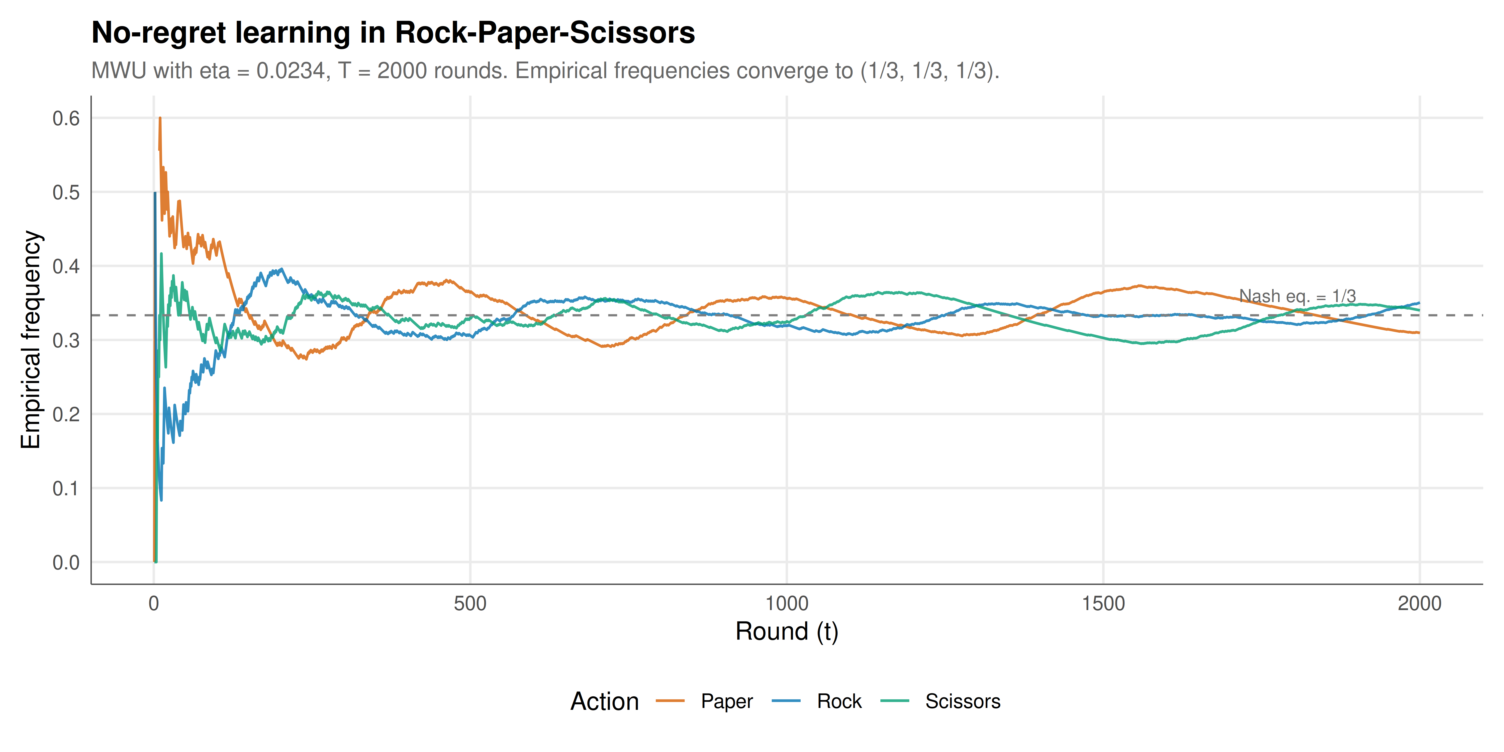
The figure tracks the empirical action frequencies of both players over time in Rock-Paper-Scissors, showing convergence to the uniform Nash equilibrium.
```{r}
#| label: fig-no-regret-static
#| fig-cap: "Figure 1. Convergence of empirical action frequencies under MWU in Rock-Paper-Scissors. Both players' time-averaged strategies converge to the Nash equilibrium (1/3, 1/3, 1/3). Initial oscillations dampen as the regret vanishes."
#| dev: [png, pdf]
#| fig-width: 10
#| fig-height: 5
#| dpi: 300
# Reshape for plotting
rps_plot <- history %>%
  select(t, p1_rock, p1_paper, p1_scissors) %>%
  pivot_longer(cols = -t, names_to = "action", values_to = "frequency") %>%
  mutate(
    action = case_when(
      action == "p1_rock" ~ "Rock",
      action == "p1_paper" ~ "Paper",
      action == "p1_scissors" ~ "Scissors"
    ),
    player = "Player 1"
  )

p_static <- ggplot(rps_plot, aes(x = t, y = frequency, colour = action)) +
  geom_line(linewidth = 0.6, alpha = 0.8) +
  geom_hline(yintercept = 1/3, linetype = "dashed", colour = "grey50", linewidth = 0.5) +
  annotate("text", x = T_rounds * 0.95, y = 0.36, label = "Nash eq. = 1/3",
           size = 3, colour = "grey40", hjust = 1) +
  scale_colour_manual(values = okabe_ito[c(6, 5, 3)], name = "Action") +
  scale_y_continuous(limits = c(0, 0.6), breaks = seq(0, 0.6, 0.1)) +
  labs(
    title = "No-regret learning in Rock-Paper-Scissors",
    subtitle = sprintf("MWU with eta = %.4f, T = %d rounds. Empirical frequencies converge to (1/3, 1/3, 1/3).", eta, T_rounds),
    x = "Round (t)", y = "Empirical frequency"
  ) +
  theme_publication()

p_static
```
## Interactive figure
The interactive figure compares the regret trajectories across the three algorithms (MWU, Exp3, FTRL) applied to Rock-Paper-Scissors.
```{r}
#| label: fig-no-regret-interactive
# Run all three algorithms and track per-round regret
T_compare <- 1000

run_algorithm <- function(algo_name, T, payoff_matrix, eta_base = NULL) {
  n_actions <- nrow(payoff_matrix)
  w1 <- rep(1, n_actions)
  w2 <- rep(1, n_actions)
  cum_payoffs_1 <- rep(0, n_actions)
  total_payoff_1 <- 0
  gamma <- 0.1  # For Exp3
  cum_utility_1 <- rep(0, n_actions)  # For FTRL

  regret_over_time <- numeric(T)

  for (t in 1:T) {
    eta <- if (!is.null(eta_base)) eta_base else sqrt(log(n_actions) / t)

    if (algo_name == "MWU") {
      s1 <- w1 / sum(w1)
      s2 <- w2 / sum(w2)
    } else if (algo_name == "Exp3") {
      s1 <- (1 - gamma) * w1 / sum(w1) + gamma / n_actions
      s2 <- (1 - gamma) * w2 / sum(w2) + gamma / n_actions
    } else {  # FTRL
      s1 <- ftrl_entropic(cum_utility_1, eta)
      s2 <- w2 / sum(w2)  # Other player uses MWU
    }

    a1 <- sample(1:n_actions, 1, prob = s1)
    a2 <- sample(1:n_actions, 1, prob = s2)

    pay1 <- payoff_matrix[a1, a2]
    total_payoff_1 <- total_payoff_1 + pay1

    payoffs_1_all <- payoff_matrix[, a2]
    payoffs_2_all <- -payoff_matrix[a1, ]

    cum_payoffs_1 <- cum_payoffs_1 + payoffs_1_all
    cum_utility_1 <- cum_utility_1 + payoffs_1_all

    if (algo_name == "MWU") {
      w1 <- mwu_update(w1, payoffs_1_all, eta)
      w2 <- mwu_update(w2, payoffs_2_all, eta)
    } else if (algo_name == "Exp3") {
      w1 <- exp3_update(w1, a1, pay1, n_actions, gamma)
      w2 <- exp3_update(w2, a2, -pay1, n_actions, gamma)
    } else {
      w2 <- mwu_update(w2, payoffs_2_all, eta)
    }

    best_fixed <- max(cum_payoffs_1)
    regret_over_time[t] <- (best_fixed - total_payoff_1) / t
  }

  data.frame(t = 1:T, per_round_regret = regret_over_time, algorithm = algo_name)
}

set.seed(42)
mwu_res  <- run_algorithm("MWU",  T_compare, rps_payoff)
set.seed(42)
exp3_res <- run_algorithm("Exp3", T_compare, rps_payoff)
set.seed(42)
ftrl_res <- run_algorithm("FTRL", T_compare, rps_payoff)
compare_data <- bind_rows(mwu_res, exp3_res, ftrl_res) %>%
  mutate(
    text = sprintf("Algorithm: %s\nRound: %d\nPer-round regret: %.4f",
                   algorithm, t, per_round_regret)
  )
p_int <- ggplot(compare_data, aes(x = t, y = per_round_regret,
                                   colour = algorithm, text = text)) +
  geom_line(linewidth = 0.6, alpha = 0.7) +
  geom_hline(yintercept = 0, linetype = "dashed", colour = "grey50") +
  scale_colour_manual(values = okabe_ito[c(5, 1, 3)], name = "Algorithm") +
  labs(
    title = "Per-round regret comparison: MWU vs. Exp3 vs. FTRL",
    subtitle = "Rock-Paper-Scissors, all algorithms converge to zero per-round regret",
    x = "Round (t)", y = "Per-round external regret"
  ) +
  theme_publication()
ggplotly(p_int, tooltip = "text") %>%
  config(displaylogo = FALSE)
```
## Interpretation
The simulation results illustrate the fundamental connection between no-regret learning and game-theoretic equilibrium in two complementary settings. In Rock-Paper-Scissors, the unique Nash equilibrium is the uniform distribution $(1/3, 1/3, 1/3)$ over all three actions. When both players use MWU, the empirical frequencies of each action converge to $1/3$ as the number of rounds increases. This convergence is not immediate --- in the early rounds, the frequencies fluctuate substantially as the algorithm explores and the weights adjust --- but the oscillations dampen over time as the learning rate effectively decreases (since we use $\eta = \sqrt{\ln K / T}$, which accounts for the full horizon). After 2000 rounds, the empirical frequencies are within a few percentage points of the equilibrium, and the per-round regret has dropped to near zero.
The convergence to a coarse correlated equilibrium (CCE) is the key theoretical guarantee. In Rock-Paper-Scissors, the set of CCE coincides with the Nash equilibrium (the uniform distribution), so convergence to CCE is equivalent to convergence to Nash. However, in general games, the set of CCE is larger than the set of Nash equilibria --- it allows for correlations between players' strategies that Nash equilibrium does not. The coordination game illustrates this: the game has two pure Nash equilibria, (A,A) and (B,B), and a mixed Nash equilibrium. The set of CCE includes all convex combinations of the equilibria plus additional correlated distributions. When both players use MWU in the coordination game, the empirical play converges to a CCE that typically involves a mixture of (A,A) and (B,B) outcomes, with the exact proportions depending on the random seed and learning dynamics. This is a weaker outcome than Nash equilibrium convergence but is the strongest guarantee that can be made for independent no-regret learners in general games.
The regret comparison across algorithms reveals important practical differences. MWU, operating in the full-information setting (where the player observes the payoffs of all actions, not just the one played), achieves the tightest regret bound and the fastest convergence. Exp3, designed for the bandit setting (where only the played action's payoff is observed), achieves sublinear regret but at a slower rate, because it must explore to estimate the payoffs of unplayed actions. The importance-weighted payoff estimates used by Exp3 introduce additional variance, which manifests as noisier regret trajectories. FTRL with entropic regularisation is mathematically equivalent to MWU in the full-information setting, and the two algorithms produce very similar regret trajectories, differing only due to implementation details and random sampling.
Several insights from no-regret learning have broader implications for game theory and mechanism design. First, the convergence to CCE rather than Nash equilibrium means that no-regret learning provides a foundation for correlated equilibrium as a prediction of game play, supporting the argument that correlated equilibrium is a more natural solution concept than Nash equilibrium for settings where players learn from experience rather than computing equilibria directly. Second, the rate of convergence ($O(\sqrt{T \ln K})$ for MWU) means that the approximation to equilibrium improves with the square root of the number of rounds, so a moderately long interaction is sufficient for approximate equilibrium to emerge. Third, the fact that each player's algorithm needs only access to their own payoffs (not other players' payoffs or strategies) means that no-regret learning is decentralised and privacy-preserving --- players can converge to equilibrium without revealing their strategies or payoff functions to each other.
There are important limitations to the no-regret convergence result. The convergence is in terms of time-averaged play, not period-by-period play. In each individual round, the players' strategies may be far from equilibrium and may exhibit cycling or chaotic behaviour, particularly in games like Rock-Paper-Scissors where the best-response dynamics are inherently cyclic. This distinction between time-average convergence and point-wise convergence has been a major focus of recent research, with some papers showing that in certain games (such as zero-sum games with certain last-iterate convergent algorithms like Optimistic MWU), point-wise convergence can also be achieved.
Furthermore, the assumption that players observe full payoff information (all counterfactual payoffs, not just the realised one) is often unrealistic. In many real-world settings, players observe only the payoff of their chosen action, corresponding to the bandit feedback model. While Exp3 handles this setting, the regret bounds are weaker, and convergence is slower. In partial monitoring settings, where even the payoff of the chosen action may be noisy or delayed, the learning problem becomes more challenging still.
Despite these caveats, no-regret learning provides one of the most compelling and practical bridges between learning theory and game theory. It demonstrates that equilibrium is not merely a theoretical construct requiring omniscient rational agents, but an emergent property of simple, adaptive learning algorithms that real agents might plausibly use.
## Extensions & related tutorials
- [Fictitious play and convergence](../../ml-and-gt/fictitious-play-convergence/) --- classical learning dynamic that predates no-regret learning and converges in certain game classes
- [Multi-agent reinforcement learning](../../ml-and-gt/multi-agent-reinforcement-learning/) --- model-free learning in games where agents do not know the payoff matrix
- [Adversarial robustness as a game](../../ml-and-gt/adversarial-robustness-games/) --- game-theoretic perspective on robustness in machine learning
- [Entropy and correlated equilibrium](../../information-theory/entropy-correlated-equilibrium/) --- information-theoretic characterisation of the correlated equilibrium set
- [Quantal response equilibrium](../../behavioral-gt/quantal-response-equilibrium/) --- equilibrium concept where players use noisy best-responses, related to the softmax in MWU
## References
::: {#refs}
:::