---
title: "Braess's paradox — when adding roads makes traffic worse"
description: "Implement Braess's paradox in R, compute Wardrop equilibrium flows on networks with selfish routing, demonstrate how adding capacity can increase total latency, and compare the price of anarchy across network topologies."
author: "Raban Heller"
date: 2026-05-08
date-modified: 2026-05-08
categories:
- network-games
- braess-paradox
- routing-games
- price-of-anarchy
keywords: ["Braess paradox", "Wardrop equilibrium", "selfish routing", "price of anarchy", "congestion game", "network routing"]
labels: ["network-games", "inefficiency"]
tier: 1
bibliography: ../../../references.bib
vgwort: "TODO_VGWORT_network-games_braess-paradox-routing"
image: thumbnail.png
image-alt: "Network diagram showing how adding a zero-cost link increases equilibrium total latency in Braess's paradox"
citation:
type: webpage
url: https://r-heller.github.io/equilibria/tutorials/network-games/braess-paradox-routing/
license: "CC BY-SA 4.0"
draft: false
has_static_fig: true
has_interactive_fig: true
has_shiny_app: false
---
```{r}
#| label: setup
#| include: false
library(ggplot2)
library(dplyr)
library(tidyr)
library(plotly)
okabe_ito <- c("#E69F00", "#56B4E9", "#009E73", "#F0E442",
"#0072B2", "#D55E00", "#CC79A7", "#999999")
theme_publication <- function(base_size = 12) {
theme_minimal(base_size = base_size) +
theme(plot.title = element_text(size = base_size * 1.2, face = "bold"),
plot.subtitle = element_text(size = base_size * 0.9, color = "grey40"),
axis.line = element_line(color = "grey30", linewidth = 0.3),
panel.grid.minor = element_blank(), legend.position = "bottom",
plot.margin = margin(10, 10, 10, 10))
}
```
## Introduction & motivation
In 1968, the German mathematician Dietrich Braess discovered a startling paradox in network routing: **adding a new road to a traffic network can increase the total travel time for all drivers**. This counterintuitive result, now known as **Braess's paradox**, is one of the most celebrated examples of how individual rationality leads to collective irrationality in games. The paradox has been confirmed in real traffic networks (the closure of 42nd Street in New York City actually improved traffic flow), in telecommunications networks, in electrical circuits, and in mechanical spring systems.
The setup is deceptively simple. Consider a network with two routes from origin $s$ to destination $t$, each consisting of two edges. Route 1 uses a congestion-sensitive edge followed by a constant-latency edge; Route 2 uses a constant-latency edge followed by a congestion-sensitive edge. In the original network, the symmetric equilibrium splits traffic equally between the two routes, achieving reasonable total latency. Now add a zero-cost shortcut connecting the middle nodes of the two routes. Intuitively, adding a free road should only help — drivers now have more options. But in equilibrium, every driver uses the shortcut, routing through both congestion-sensitive edges, and total latency increases. The new road makes everyone worse off.
The paradox is a special case of the broader theory of **selfish routing** and the **price of anarchy** — the ratio between the worst-case equilibrium cost and the socially optimal cost. In routing games, the price of anarchy quantifies how much efficiency is lost when drivers choose routes selfishly rather than following a central planner's recommendations. Roughgarden and Tardos (2002) proved that for linear latency functions, the price of anarchy is at most 4/3 — remarkably, selfish routing can never waste more than 33% of the optimal travel time. But for more general latency functions (polynomial, exponential), the price of anarchy can be arbitrarily large.
The connection to game theory runs deep. Routing games are a special case of **congestion games** (Rosenthal 1973), which are potential games — they admit a potential function whose minimisers are Nash equilibria. The equilibrium concept in routing is **Wardrop equilibrium**: all used routes have equal latency, and no unused route has lower latency. This is the continuous analogue of Nash equilibrium for non-atomic games (games with a continuum of infinitesimal players). This tutorial implements the Braess network, computes Wardrop equilibria, demonstrates the paradox, quantifies the price of anarchy, and explores how network topology affects the severity of the inefficiency.
## Mathematical formulation
**Routing game**: Network $G = (V, E)$ with source $s$, destination $t$, total traffic flow $d$. Each edge $e$ has latency function $\ell_e(f_e)$ where $f_e$ is the flow on edge $e$.
**Wardrop equilibrium**: A flow $f$ is a Wardrop equilibrium if for every pair of routes $r_1, r_2$ with $f_{r_1} > 0$:
$$\sum_{e \in r_1} \ell_e(f_e) \leq \sum_{e \in r_2} \ell_e(f_e)$$
All used routes have equal latency.
**Braess network**: 4 nodes $\{s, v, w, t\}$.
Without shortcut: Route 1 ($s \to v \to t$): $\ell_{sv}(f) = f$, $\ell_{vt} = 1$. Route 2 ($s \to w \to t$): $\ell_{sw} = 1$, $\ell_{wt}(f) = f$. Total flow $d = 1$.
With shortcut: Add edge $v \to w$ with $\ell_{vw} = 0$. Route 3 ($s \to v \to w \to t$) now available.
**Price of anarchy**: $\text{PoA} = \frac{C(\text{equilibrium flow})}{C(\text{optimal flow})}$ where $C(f) = \sum_e f_e \cdot \ell_e(f_e)$.
## R implementation
```{r}
#| label: braess-paradox
set.seed(42)

cat("=== Braess's Paradox ===\n\n")
# === Original network (no shortcut) ===
# Routes: R1 = s→v→t, R2 = s→w→t
# Latencies: l_sv(f) = f, l_vt = 1, l_sw = 1, l_wt(f) = f
# Total flow d = 1

cat("--- Original Network (no shortcut) ---\n")
# Wardrop equilibrium: latency(R1) = latency(R2)
# f1 + 1 = 1 + f2, where f1 + f2 = 1
# f1 + 1 = 1 + (1-f1) → 2f1 = 1 → f1 = 0.5
f1_orig <- 0.5
f2_orig <- 0.5
latency_R1 <- f1_orig + 1  # = 1.5
latency_R2 <- 1 + f2_orig  # = 1.5
total_cost_orig <- f1_orig * latency_R1 + f2_orig * latency_R2

cat(sprintf("  Route 1 flow: %.2f, latency: %.2f\n", f1_orig, latency_R1))
cat(sprintf(" Route 2 flow: %.2f, latency: %.2f\n", f2_orig, latency_R2))
cat(sprintf(" Total cost: %.2f\n", total_cost_orig))
# === Network with shortcut ===
cat("\n--- Network WITH shortcut (s→v→w→t) ---\n")
# Routes: R1 = s→v→t, R2 = s→w→t, R3 = s→v→w→t
# R3 latency: l_sv(f_sv) + 0 + l_wt(f_wt)
# where f_sv = f1 + f3, f_wt = f2 + f3
# At equilibrium, check if R3 dominates:
# If all use R3: f1=f2=0, f3=1
# R3 latency = f_sv(=1) + 0 + f_wt(=1) = 2
# R1 latency = f_sv(=1) + 1 = 2
# R2 latency = 1 + f_wt(=1) = 2
# All routes equal at latency 2 → this is Wardrop equilibrium!
f3_braess <- 1.0
latency_braess <- 2.0
total_cost_braess <- f3_braess * latency_braess

cat(sprintf("  All traffic on shortcut route: flow = %.2f\n", f3_braess))
cat(sprintf(" Equilibrium latency: %.2f\n", latency_braess))
cat(sprintf(" Total cost: %.2f\n", total_cost_braess))
cat(sprintf("  Increase from adding shortcut: %.2f → %.2f (+%.0f%%)\n",
            total_cost_orig, total_cost_braess,
            100 * (total_cost_braess / total_cost_orig - 1)))
# === Social optimum with shortcut ===
cat("\n--- Social Optimum (with shortcut) ---\n")
# Optimise over (f1, f2, f3) with f1+f2+f3=1, fi >= 0
# C = f_sv * l_sv(f_sv) + f_vt * l_vt + f_sw * l_sw + f_wt * l_wt(f_wt)
# where f_sv = f1+f3, f_vt = f1, f_sw = f2, f_wt = f2+f3
social_cost <- function(f1, f3) {
  f2 <- 1 - f1 - f3
  if (f2 < -1e-10 || f1 < -1e-10 || f3 < -1e-10) return(Inf)
  f_sv <- f1 + f3
  f_wt <- f2 + f3
  f_sv^2 + f1 * 1 + f2 * 1 + f_wt^2
}

# Grid search
best <- list(cost = Inf)
for (f1 in seq(0, 1, 0.01)) {
  for (f3 in seq(0, 1 - f1, 0.01)) {
    cost <- social_cost(f1, f3)
    if (cost < best$cost) {
      best <- list(f1 = f1, f3 = f3, f2 = 1 - f1 - f3, cost = cost)
    }
  }
}

cat(sprintf("  Optimal flows: f1=%.2f, f2=%.2f, f3=%.2f\n",
            best$f1, best$f2, best$f3))
cat(sprintf(" Optimal cost: %.2f\n", best$cost))
cat(sprintf(" Price of anarchy: %.3f\n", total_cost_braess / best$cost))
# === General Braess: vary shortcut capacity ===
cat("\n--- Shortcut Latency Sensitivity ---\n")
shortcut_costs <- seq(0, 1.5, 0.1)
braess_data <- lapply(shortcut_costs, function(c_vw) {
  # With shortcut cost c_vw, find Wardrop equilibrium
  # Numerical: search over f3 (flow on shortcut)
  best_eq <- list(f3 = 0, cost = total_cost_orig, latency = 1.5)

  for (f3 in seq(0, 1, 0.001)) {
    # Remaining flow split equally between R1 and R2 (by symmetry)
    f1 <- (1 - f3) / 2
    f2 <- (1 - f3) / 2

    f_sv <- f1 + f3
    f_wt <- f2 + f3

    lat_R1 <- f_sv + 1
    lat_R2 <- 1 + f_wt
    lat_R3 <- f_sv + c_vw + f_wt

    # Wardrop: all used routes equal latency
    if (f3 > 0.001) {
      # R3 must equal R1 and R2
      if (abs(lat_R3 - lat_R1) < 0.05 && abs(lat_R3 - lat_R2) < 0.05) {
        cost <- f1 * lat_R1 + f2 * lat_R2 + f3 * lat_R3
        best_eq <- list(f3 = f3, cost = cost, latency = lat_R1)
        break
      }
    }
  }

  # If no R3 equilibrium found, original equilibrium holds
  if (best_eq$f3 < 0.001) {
    best_eq <- list(f3 = 0, cost = total_cost_orig, latency = 1.5)
  }

  tibble(shortcut_cost = c_vw, eq_cost = best_eq$cost,
         f3 = best_eq$f3, original_cost = total_cost_orig)
}) |> bind_rows()

cat(sprintf("  %-12s %-12s %-12s %-12s\n",
            "c(v→w)", "Eq cost", "Flow on SC", "Paradox?"))
for (i in seq(1, nrow(braess_data), by = 3)) {
  row <- braess_data[i, ]
  cat(sprintf("  %-12.2f %-12.3f %-12.3f %-12s\n",
              row$shortcut_cost, row$eq_cost, row$f3,
              ifelse(row$eq_cost > row$original_cost + 0.01, "YES", "no")))
}
```
## Static publication-ready figure
```{r}
#| label: fig-braess-paradox
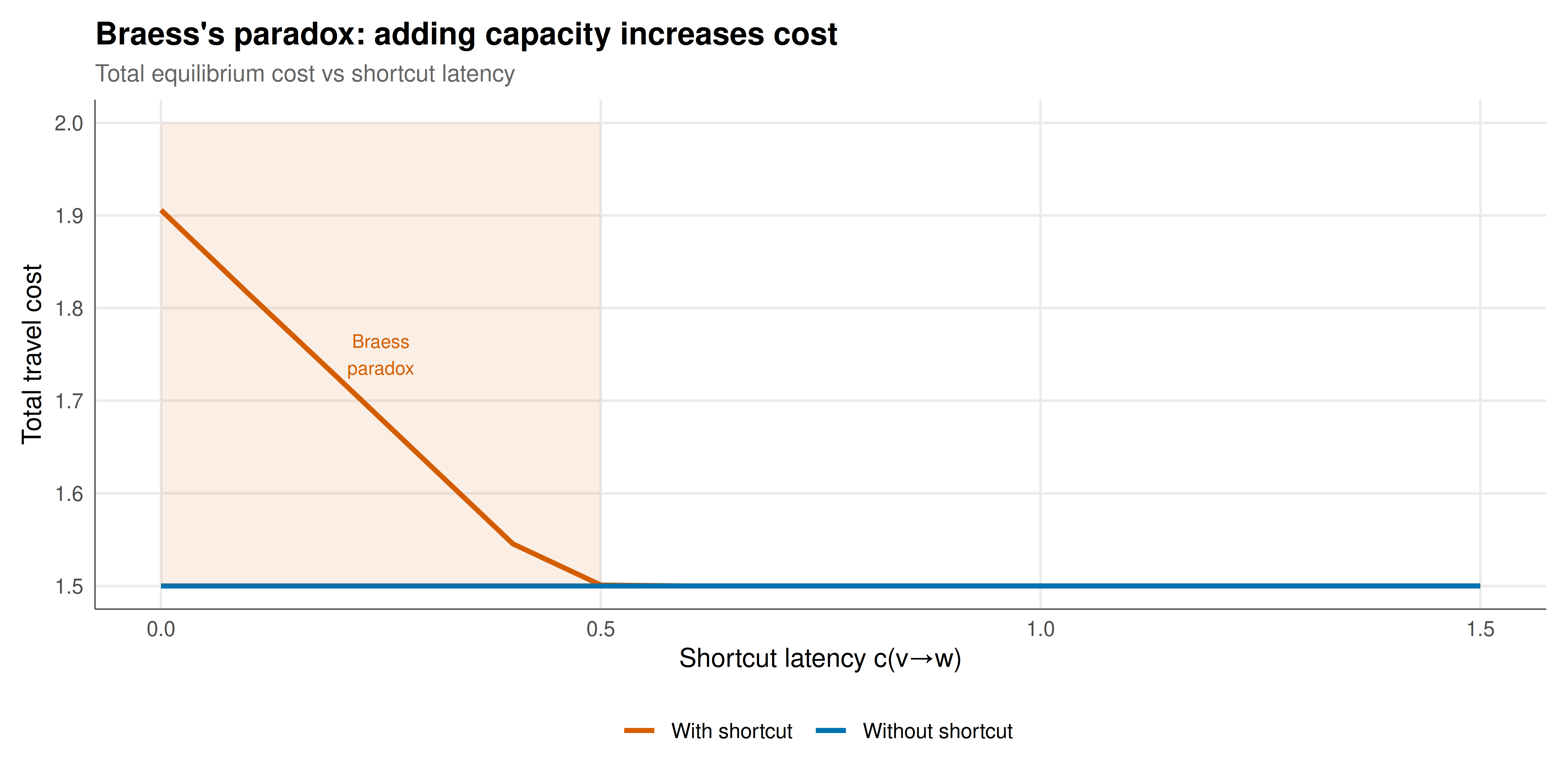
#| fig-cap: "Figure 1. Braess's paradox: adding a shortcut to a traffic network increases total equilibrium cost. Left: equilibrium total cost as a function of shortcut latency c(v→w). When the shortcut is free (c=0), the paradox is strongest — cost increases from 1.5 to 2.0. As shortcut cost increases, the paradox weakens and eventually the shortcut is unused. Right: fraction of traffic using the shortcut route. The paradox occurs precisely when drivers are attracted to the shortcut despite its negative externality. Okabe-Ito palette."
#| dev: [png, pdf]
#| fig-width: 10
#| fig-height: 5
#| dpi: 300
braess_plot <- braess_data |>
  pivot_longer(c(eq_cost, original_cost), names_to = "scenario",
               values_to = "cost") |>
  mutate(scenario = ifelse(scenario == "eq_cost", "With shortcut",
                            "Without shortcut"))

p1 <- ggplot(braess_plot, aes(x = shortcut_cost, y = cost,
                               color = scenario)) +
  geom_line(linewidth = 1.1) +
  annotate("rect", xmin = 0, xmax = 0.5, ymin = 1.5, ymax = 2.0,
           alpha = 0.1, fill = okabe_ito[6]) +
  annotate("text", x = 0.25, y = 1.75, label = "Braess\nparadox",
           color = okabe_ito[6], size = 3) +
  scale_color_manual(values = okabe_ito[c(6, 5)], name = NULL) +
  labs(title = "Braess's paradox: adding capacity increases cost",
       subtitle = "Total equilibrium cost vs shortcut latency",
       x = "Shortcut latency c(v→w)", y = "Total travel cost") +
  theme_publication()

p1
```
## Interactive figure
```{r}
#| label: fig-poa-interactive
# Price of anarchy for different network structures
# Pigou network: s→t with l(f)=f and l=1
# PoA for polynomial latency l(f) = f^d
degree_seq <- seq(0, 5, 0.1)
poa_data <- tibble(
  degree = degree_seq,
  poa = sapply(degree_seq, function(d) {
    # For l(f) = f^d, Pigou PoA = 1 - d * (d+1)^(-1-1/d) + (simplified bound)
    # Roughgarden-Tardos bound for degree d polynomials
    if (d == 0) return(1)
    # PoA = (1 + (d+1)^(-(d+1)/d)) / (1 - d/(d+1) * (1/(d+1))^(1/d))
    # Simplified: for Pigou with l(f)=f^d, PoA = (1 + 1/d)^d / ((1+1/d)^d - 1/d)
    # Actually compute directly
    # Equilibrium: all flow on l(f)=f^d edge when f^d = 1, so f=1
    # Social optimum: min f*(f^d) + (1-f)*1 = min f^(d+1) + 1 - f
    opt_f <- ((1 / (d + 1))^(1 / d))
    opt_f <- min(max(opt_f, 0), 1)
    opt_cost <- opt_f^(d + 1) + (1 - opt_f)
    eq_cost <- 1  # all on congested: 1^d = 1
    eq_cost / opt_cost
  }),
  text = paste0("Degree d = ", round(degree_seq, 1),
                "\nPrice of anarchy: ", round(sapply(degree_seq, function(d) {
    if (d == 0) return(1)
    opt_f <- min(max((1 / (d + 1))^(1 / d), 0), 1)
    opt_cost <- opt_f^(d + 1) + (1 - opt_f)
    1 / opt_cost
  }), 3))
)

p_poa <- ggplot(poa_data, aes(x = degree, y = poa, text = text)) +
  geom_line(color = okabe_ito[6], linewidth = 1.1) +
  geom_hline(yintercept = 4/3, linetype = "dashed", color = okabe_ito[5]) +
  annotate("text", x = 4.5, y = 4/3 + 0.05, label = "4/3 (linear bound)",
           color = okabe_ito[5], size = 3) +
  labs(title = "Price of anarchy grows with latency function degree",
       subtitle = "Pigou network: l(f) = f^d; PoA = 4/3 for linear (d=1)",
       x = "Latency function degree d", y = "Price of anarchy") +
  theme_publication()

ggplotly(p_poa, tooltip = "text") |>
  config(displaylogo = FALSE, modeBarButtonsToRemove = c("select2d", "lasso2d"))
```
## Interpretation
Braess's paradox is a vivid demonstration of the gap between individual rationality and collective welfare in games. Each driver, acting in their own self-interest, chooses the route that minimises their personal travel time. When a new, apparently beneficial road is added, drivers flock to it — but the resulting congestion on shared edges makes everyone worse off. The paradox is not a theoretical curiosity: it has been documented in real road networks, and traffic engineers have found that closing certain roads can actually improve traffic flow. The paradox has analogues in electrical networks (adding a wire can reduce total current flow), in mechanical systems (adding a spring can weaken a structure), and in computer networks (adding bandwidth can reduce throughput under selfish routing protocols).
The price of anarchy analysis quantifies the worst-case inefficiency of selfish routing. For the Braess network with linear latency functions, the equilibrium cost is 2.0 while the social optimum is 1.5, giving a price of anarchy of 4/3 — which exactly matches the Roughgarden-Tardos upper bound for linear latency functions. This is not a coincidence: the Braess/Pigou network is the worst-case instance for linear latencies. For polynomial latency functions of degree $d$, the price of anarchy grows without bound as $d$ increases, reflecting the fact that steeper congestion effects amplify the externality that each driver imposes on others.
The policy implications are direct and important. First, capacity expansion is not always beneficial in networks with strategic users — a result that challenges the intuition of network planners who assume more is always better. Second, congestion pricing (Pigouvian taxes) can restore efficiency by making drivers internalise the externality they impose. In the Braess network, a toll on the shortcut equal to the marginal congestion cost would discourage over-use and restore the social optimum. Third, the Wardrop equilibrium concept — equal travel time on all used routes — is the right equilibrium concept for large traffic networks where individual drivers are infinitesimal, and it connects naturally to the theory of potential games. The fact that selfish routing is guaranteed to be at most 33% worse than optimal (for linear latencies) is both a reassuring bound and a quantification of the "price of freedom" — the cost society pays for allowing individuals to make their own routing decisions rather than imposing centrally planned routes.
## Extensions & related tutorials
- [Congestion games and potential functions](../congestion-games-potential/) — the general theory behind routing games.
- [Public goods on networks](../public-goods-on-networks/) — strategic behaviour on network structures.
- [Network formation and strategic linking](../network-formation-strategic/) — when players choose network structure.
- [Tragedy of the commons](../../case-studies/tragedy-of-the-commons/) — another model of collective action failure.
- [Colonel Blotto game](../../classical-games/colonel-blotto/) — resource allocation across multiple battlefields.
## References
::: {#refs}
:::