Diffusion and cascades on networks

Simulate information cascades using the linear threshold and independent cascade models on random networks, demonstrating tipping points and the effect of network structure on cascade size.

Keywords

information cascades, linear threshold model, independent cascade, tipping point, network diffusion, igraph, R

Introduction & motivation

When a new technology, idea, or behaviour spreads through a population, it rarely happens uniformly. Instead, adoption typically follows a cascade pattern: a small number of early adopters trigger their neighbours to adopt, who in turn trigger their neighbours, and so on. Whether the cascade reaches a large fraction of the population or fizzles out after a few steps depends critically on the structure of the underlying social network and the local adoption rules. Understanding these cascades is central to viral marketing, epidemiology, the spread of political movements, and the diffusion of innovations more broadly.

From a game-theoretic perspective, adoption cascades can be modelled as coordination games on networks. Each node in the network is a player who must choose between two actions (e.g., adopt or not adopt a new technology). The payoff from adoption increases with the number of neighbours who also adopt, creating strategic complementarities. A node will switch to adoption when a sufficient fraction of its neighbours have already adopted – this is the essence of the linear threshold model (LTM), introduced by Granovetter (1978) and formalised for networks by Kempe, Kleinberg, and Tardos (2003). The LTM assigns each node a random threshold \(\theta_i \in [0, 1]\); node \(i\) adopts when the fraction of its neighbours who have adopted exceeds \(\theta_i\).

An alternative model is the independent cascade model (ICM), where each newly adopted node gets a single chance to independently “infect” each of its not-yet-adopted neighbours with some probability \(p\). The ICM is equivalent to bond percolation on the network and is closely related to epidemiological SIR models. Both models capture different aspects of real-world diffusion: the LTM emphasises social influence and threshold behaviour, while the ICM emphasises probabilistic transmission.

A key phenomenon in both models is the tipping point: there exists a critical seed size (or critical network density) below which cascades are small and localised, and above which a small perturbation can trigger a global cascade affecting a large fraction of the network. This phase transition is sharper in some network topologies than others. On Erdos-Renyi random graphs, the tipping point is closely related to the giant component threshold. On scale-free networks (with power-law degree distributions), the structure is richer: high-degree hub nodes can act as super-spreaders, but they are also harder to activate because their thresholds require more absolute neighbours to adopt.

In this tutorial, we implement both the linear threshold model and the independent cascade model on random graphs generated with igraph. We simulate cascades on Erdos-Renyi and scale-free (Barabasi-Albert) networks, systematically vary seed size and network density, and visualise the cascade size to identify tipping points and compare network topologies.

Mathematical formulation

Let \(G = (V, E)\) be an undirected network with \(|V| = n\) nodes. Define:

Linear Threshold Model (LTM):

1. Each node \(i\) draws a threshold \(\theta_i \sim \text{Uniform}[0, 1]\) independently.
2. A seed set \(S_0 \subseteq V\) of initially active nodes is chosen.
3. At each step \(t\), an inactive node \(i\) becomes active if:

\[ \frac{|\{j \in N(i) : j \text{ is active}\}|}{|N(i)|} \geq \theta_i \]

where \(N(i)\) is the set of neighbours of \(i\). The process terminates when no new nodes activate.

Independent Cascade Model (ICM):

1. A seed set \(S_0\) is chosen and a transmission probability \(p \in [0, 1]\) is fixed.
2. When node \(i\) first becomes active at time \(t\), it attempts to activate each inactive neighbour \(j\) independently with probability \(p\).
3. Regardless of success, \(i\) does not attempt to activate \(j\) again. The process terminates when no new activations occur.

Cascade size is defined as the fraction of nodes that are active at termination:

\[ \text{Cascade fraction} = \frac{|S_\infty|}{n} \]

Tipping point: In the LTM on Erdos-Renyi graphs \(G(n, p_{\text{edge}})\) with uniform thresholds, a global cascade (affecting a constant fraction of \(n\)) occurs when the mean degree \(\langle k \rangle = (n-1) p_{\text{edge}}\) and seed fraction interact to cross a critical boundary. The condition for cascade propagation is roughly that a node with degree \(k\) will adopt when \(\theta_i < s\) (seed fraction among neighbours), which requires:

\[ \sum_{k} P(k) \cdot P\left(\theta < \frac{1}{k}\right) > 1 \]

for the cascade to be self-sustaining (analogous to \(R_0 > 1\) in epidemiology).

R implementation

We implement both models and run systematic simulations on Erdos-Renyi and Barabasi-Albert networks.

# --- Linear Threshold Model ---
run_ltm <- function(g, seed_nodes, thresholds = NULL) {
  n <- vcount(g)
  if (is.null(thresholds)) {
    thresholds <- runif(n)
  }

  active <- rep(FALSE, n)
  active[seed_nodes] <- TRUE
  newly_active <- seed_nodes

  while (length(newly_active) > 0) {
    candidates <- unique(unlist(neighborhood(g, order = 1,
                                             nodes = newly_active)))
    candidates <- candidates[!active[candidates]]

    if (length(candidates) == 0) break

    newly_active <- integer(0)
    for (node in candidates) {
      nbrs <- neighbors(g, node)
      frac_active <- sum(active[nbrs]) / length(nbrs)
      if (frac_active >= thresholds[node]) {
        newly_active <- c(newly_active, node)
      }
    }

    active[newly_active] <- TRUE
  }

  sum(active) / n
}

# --- Independent Cascade Model ---
run_icm <- function(g, seed_nodes, prob = 0.1) {
  n <- vcount(g)
  active <- rep(FALSE, n)
  active[seed_nodes] <- TRUE
  newly_active <- seed_nodes

  while (length(newly_active) > 0) {
    next_active <- integer(0)
    for (node in newly_active) {
      nbrs <- neighbors(g, node)
      inactive_nbrs <- nbrs[!active[nbrs]]
      if (length(inactive_nbrs) > 0) {
        transmit <- rbinom(length(inactive_nbrs), 1, prob) == 1
        next_active <- c(next_active, inactive_nbrs[transmit])
      }
    }
    next_active <- unique(next_active)
    next_active <- next_active[!active[next_active]]
    active[next_active] <- TRUE
    newly_active <- next_active
  }

  sum(active) / n
}

# --- Simulation parameters ---
set.seed(42)
n_nodes <- 200
n_reps <- 30
seed_fracs <- seq(0.01, 0.15, by = 0.01)

# Erdos-Renyi networks at different densities
er_densities <- c(0.03, 0.05, 0.08)

cat("=== Linear Threshold Model on Erdos-Renyi Networks ===\n")

=== Linear Threshold Model on Erdos-Renyi Networks ===

ltm_results <- data.frame()

for (p_edge in er_densities) {
  for (sf in seed_fracs) {
    cascade_sizes <- numeric(n_reps)
    for (rep in 1:n_reps) {
      g <- erdos.renyi.game(n_nodes, p_edge, type = "gnp")
      seed_size <- max(1, round(sf * n_nodes))
      seeds <- sample(1:n_nodes, seed_size)
      cascade_sizes[rep] <- run_ltm(g, seeds)
    }
    ltm_results <- rbind(ltm_results, data.frame(
      seed_frac = sf,
      cascade_frac = mean(cascade_sizes),
      cascade_sd = sd(cascade_sizes),
      density = paste0("p = ", p_edge),
      model = "LTM",
      network = "Erdos-Renyi"
    ))
  }
}

cat("Mean degree for each density:\n")

Mean degree for each density:

for (p in er_densities) {
  cat(sprintf("  p = %.2f: <k> = %.1f\n", p, (n_nodes - 1) * p))
}

  p = 0.03: <k> = 6.0
  p = 0.05: <k> = 10.0
  p = 0.08: <k> = 15.9

# Compare Erdos-Renyi vs Barabasi-Albert for ICM
cat("\n=== Independent Cascade Model: ER vs BA Networks ===\n")

=== Independent Cascade Model: ER vs BA Networks ===

icm_results <- data.frame()
icm_prob <- 0.08

for (sf in seed_fracs) {
  # Erdos-Renyi
  cascade_er <- numeric(n_reps)
  cascade_ba <- numeric(n_reps)
  for (rep in 1:n_reps) {
    g_er <- erdos.renyi.game(n_nodes, 0.05, type = "gnp")
    g_ba <- barabasi.game(n_nodes, m = 5, directed = FALSE)
    seed_size <- max(1, round(sf * n_nodes))
    seeds_er <- sample(1:n_nodes, seed_size)
    seeds_ba <- sample(1:n_nodes, seed_size)
    cascade_er[rep] <- run_icm(g_er, seeds_er, prob = icm_prob)
    cascade_ba[rep] <- run_icm(g_ba, seeds_ba, prob = icm_prob)
  }
  icm_results <- rbind(icm_results, data.frame(
    seed_frac = rep(sf, 2),
    cascade_frac = c(mean(cascade_er), mean(cascade_ba)),
    cascade_sd = c(sd(cascade_er), sd(cascade_ba)),
    network = c("Erdos-Renyi", "Barabasi-Albert"),
    model = "ICM"
  ))
}

cat("ICM transmission probability:", icm_prob, "\n")

ICM transmission probability: 0.08 

cat("\nSample results (seed fraction = 0.05):\n")

Sample results (seed fraction = 0.05):

print(icm_results %>% filter(abs(seed_frac - 0.05) < 0.001) %>%
        select(network, cascade_frac, cascade_sd))

          network cascade_frac cascade_sd
1     Erdos-Renyi       0.1705 0.07402644
2 Barabasi-Albert       0.2315 0.08421186

Static publication-ready figure

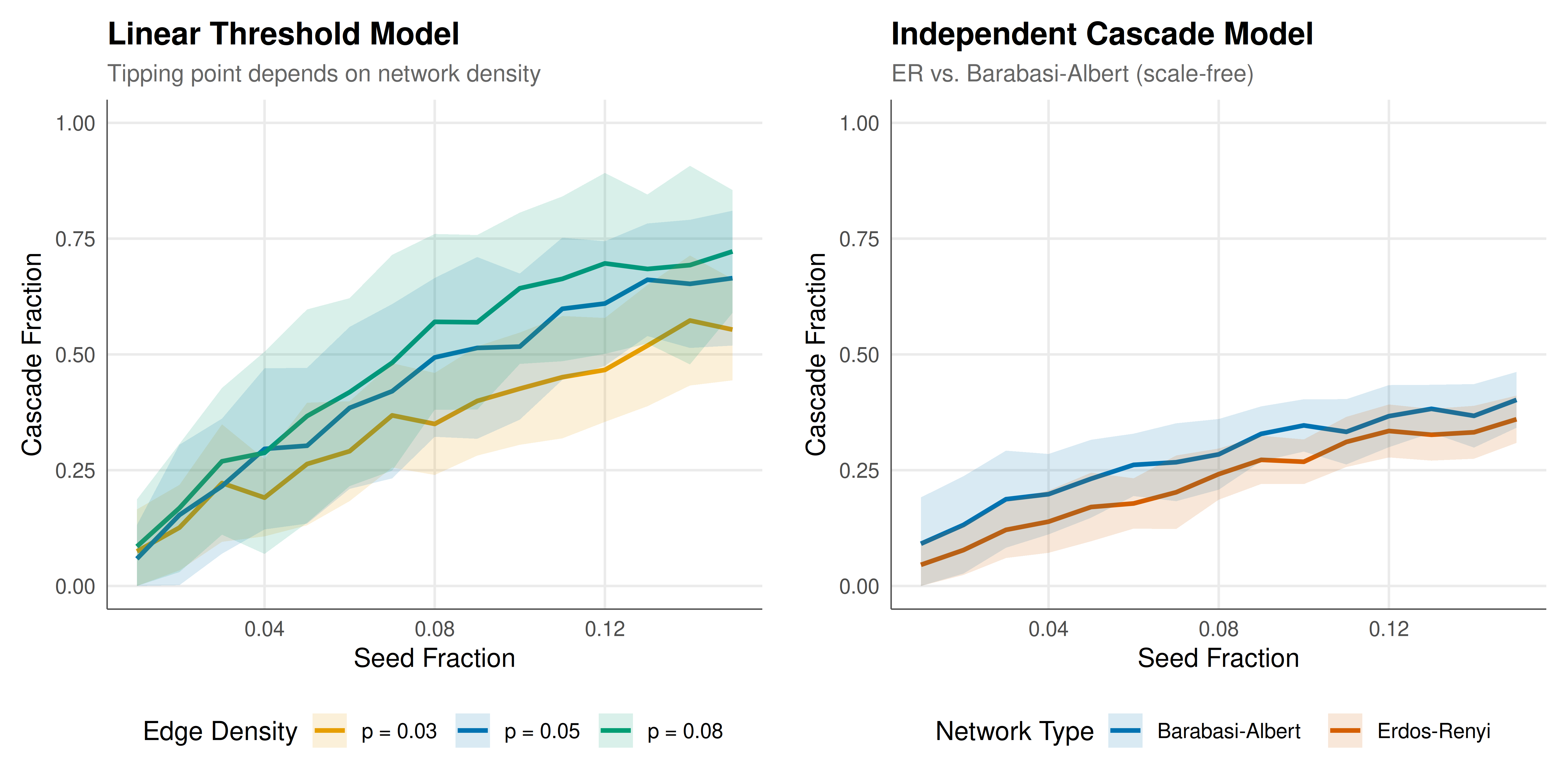
We create a two-panel figure: the left panel shows the LTM cascade size as a function of seed fraction for different network densities (showing the tipping point), and the right panel compares ICM cascades on Erdos-Renyi vs. Barabasi-Albert networks.

p_ltm <- ggplot(ltm_results,
                aes(x = seed_frac, y = cascade_frac, color = density)) +
  geom_line(linewidth = 1.0) +
  geom_ribbon(aes(ymin = pmax(0, cascade_frac - cascade_sd),
                  ymax = pmin(1, cascade_frac + cascade_sd),
                  fill = density),
              alpha = 0.15, color = NA) +
  scale_color_manual(values = okabe_ito[c(1, 5, 3)], name = "Edge Density") +
  scale_fill_manual(values = okabe_ito[c(1, 5, 3)], name = "Edge Density") +
  labs(
    title = "Linear Threshold Model",
    subtitle = "Tipping point depends on network density",
    x = "Seed Fraction", y = "Cascade Fraction"
  ) +
  theme_publication() +
  coord_cartesian(ylim = c(0, 1))

p_icm <- ggplot(icm_results,
                aes(x = seed_frac, y = cascade_frac, color = network)) +
  geom_line(linewidth = 1.0) +
  geom_ribbon(aes(ymin = pmax(0, cascade_frac - cascade_sd),
                  ymax = pmin(1, cascade_frac + cascade_sd),
                  fill = network),
              alpha = 0.15, color = NA) +
  scale_color_manual(values = okabe_ito[c(5, 6)], name = "Network Type") +
  scale_fill_manual(values = okabe_ito[c(5, 6)], name = "Network Type") +
  labs(
    title = "Independent Cascade Model",
    subtitle = "ER vs. Barabasi-Albert (scale-free)",
    x = "Seed Fraction", y = "Cascade Fraction"
  ) +
  theme_publication() +
  coord_cartesian(ylim = c(0, 1))

gridExtra::grid.arrange(p_ltm, p_icm, ncol = 2)

Figure 1: Figure 1. Cascade dynamics on random networks. Left: Linear threshold model on Erdos-Renyi networks of varying density – denser networks exhibit a sharper tipping point. Right: Independent cascade model comparing Erdos-Renyi and Barabasi-Albert topologies, showing how scale-free structure affects diffusion.

Interactive figure

The interactive figure lets readers explore the LTM results in detail, with tooltips showing the exact seed fraction, cascade fraction, and standard deviation for each data point.

ltm_int <- ltm_results %>%
  mutate(label = sprintf(
    "Density: %s\nSeed fraction: %.2f\nCascade fraction: %.3f\nSD: %.3f",
    density, seed_frac, cascade_frac, cascade_sd
  ))

p_int <- ggplot(ltm_int,
                aes(x = seed_frac, y = cascade_frac, color = density,
                    text = label)) +
  geom_line(linewidth = 0.9) +
  geom_point(size = 2, alpha = 0.7) +
  scale_color_manual(values = okabe_ito[c(1, 5, 3)], name = "Edge Density") +
  labs(
    title = "Linear Threshold Model: Cascade Size vs. Seed Fraction",
    x = "Seed Fraction", y = "Cascade Fraction"
  ) +
  theme_publication() +
  coord_cartesian(ylim = c(0, 1))

ggplotly(p_int, tooltip = "text") %>%
  config(displaylogo = FALSE)

Figure 2

Interpretation

The simulation results reveal several key insights about diffusion dynamics on networks. In the linear threshold model, the cascade size exhibits a clear tipping point as a function of seed fraction. For sparse networks (low edge probability \(p = 0.03\)), even a relatively large seed set fails to trigger a global cascade because nodes have too few connections for the influence to propagate. As network density increases (\(p = 0.05\) and \(p = 0.08\)), the tipping point becomes both lower (smaller seeds can trigger large cascades) and sharper (the transition from small to large cascade is more abrupt). This is directly analogous to the phase transition in percolation theory and the epidemic threshold in SIR models.

The denser networks support larger cascades because higher mean degree \(\langle k \rangle\) means each active node has more neighbours to influence. However, there is a subtle non-monotonicity in the LTM: when networks are very dense, each node has many neighbours, so a node with threshold \(\theta\) needs a larger absolute number of active neighbours to be triggered. This can sometimes make dense networks more resistant to early-stage cascades while supporting larger cascades once the tipping point is crossed. The standard deviation bands in our plots capture this variability, which is highest near the tipping point where small differences in network structure or seed placement lead to vastly different outcomes.

The comparison between Erdos-Renyi and Barabasi-Albert networks under the independent cascade model reveals the role of degree heterogeneity. Scale-free networks (Barabasi-Albert) have hub nodes with very high degree, which can act as super-spreaders: once a hub is activated, it attempts to infect many neighbours simultaneously. However, hubs are also initially harder to influence in the LTM because they require a larger fraction of their many neighbours to be active. In the ICM, the effect is more straightforward: hubs amplify cascades, leading to generally larger cascade sizes at the same seed fraction compared to Erdos-Renyi networks with similar average degree.

These findings have practical implications. For viral marketing, they suggest that targeting strategies should account for network structure: seeding a few hub nodes in a scale-free network may be more effective than random seeding. For network resilience, the results suggest that networks near the tipping point are especially fragile – a small increase in initial adoption can tip the system into a global cascade. This sensitivity has implications for managing both desirable cascades (innovation adoption) and undesirable ones (misinformation, epidemics).

Extensions & related tutorials

Network cascades connect to many areas of game theory and network science. The influence maximisation problem asks which seed set maximises expected cascade size, and is NP-hard but admits a greedy approximation with provable guarantees. Evolutionary game theory on networks studies how strategies spread through local interactions. The price of anarchy in network routing connects congestion games to network structure.

• Congestion games and potential functions
• Fictitious play and convergence
• Value of information in strategic games
• Support enumeration algorithm for Nash equilibria

References