---
title: "Power-law networks and strategic behaviour"
description: "Analyse how scale-free degree distributions in Barabasi-Albert networks affect coordination game outcomes, hub influence on equilibrium selection, and targeted vs random intervention strategies using R simulations."
author: "Raban Heller"
date: 2026-05-08
date-modified: 2026-05-08
categories:
- network-science
- scale-free-networks
- coordination-games
- network-interventions
keywords: ["scale-free network", "Barabasi-Albert", "power-law", "coordination game", "hub influence", "network intervention", "vaccination", "equilibrium selection", "Erdos-Renyi"]
labels: ["network-science", "simulations"]
tier: 1
bibliography: ../../../references.bib
vgwort: "TODO_VGWORT_network-science_power-law-networks-strategic"
image: thumbnail.png
image-alt: "Comparison of adoption curves on scale-free versus Erdos-Renyi networks showing faster convergence when hubs are targeted"
citation:
type: webpage
url: https://r-heller.github.io/equilibria/tutorials/network-science/power-law-networks-strategic/
license: "CC BY-SA 4.0"
draft: false
has_static_fig: true
has_interactive_fig: true
has_shiny_app: false
---
```{r}
#| label: setup
#| include: false
library(ggplot2)
library(dplyr)
library(tidyr)
library(plotly)
library(igraph)
okabe_ito <- c("#E69F00", "#56B4E9", "#009E73", "#F0E442",
"#0072B2", "#D55E00", "#CC79A7", "#999999")
theme_publication <- function(base_size = 12) {
theme_minimal(base_size = base_size) +
theme(plot.title = element_text(size = base_size * 1.2, face = "bold"),
plot.subtitle = element_text(size = base_size * 0.9, color = "grey40"),
axis.line = element_line(color = "grey30", linewidth = 0.3),
panel.grid.minor = element_blank(), legend.position = "bottom",
plot.margin = margin(10, 10, 10, 10))
}
```
## Introduction & motivation
Many real-world networks --- social networks, the internet, citation networks, protein interaction networks --- exhibit degree distributions that follow a power law: the probability that a node has degree $k$ scales as $P(k) \propto k^{-\gamma}$, typically with $2 < \gamma < 3$. This means that while most nodes have few connections, a small number of "hubs" have extraordinarily many. These scale-free networks, first modelled by Barabasi and Albert through preferential attachment, have structural properties dramatically different from the homogeneous Erdos-Renyi random graphs that had dominated network science for decades.
The implications for strategic behaviour are profound. When agents play games on networks --- choosing strategies based on the behaviour of their neighbours --- the heterogeneous degree distribution of a scale-free network creates asymmetric strategic environments. A hub node that adopts a particular strategy exerts influence on dozens or hundreds of neighbours, while a peripheral node influences only a handful. In a coordination game, where players want to match their neighbours' strategies, this means that hubs serve as de facto leaders of equilibrium selection: if a hub switches to strategy B, its many neighbours suddenly face strong pressure to follow, potentially triggering a cascade of adoption across the network.
This asymmetry has direct practical consequences. Consider a public health campaign aiming to promote vaccination (a coordination-like game where the benefit of vaccinating increases with the number of vaccinated neighbours). On a scale-free network, targeting hubs for vaccination --- rather than vaccinating random individuals --- is dramatically more effective at reaching herd immunity. This "targeted intervention" strategy exploits the network structure: by converting the most-connected nodes, you influence the maximum number of neighbours per intervention dollar spent.
In this tutorial, we generate Barabasi-Albert scale-free networks and Erdos-Renyi random networks, verify their degree distributions, and then simulate a coordination game played on both network types. We measure how quickly the population converges to an equilibrium, how hubs influence which equilibrium is selected, and how targeted versus random intervention strategies differ in their effectiveness. The results demonstrate that network topology is not merely a backdrop for strategic interaction but a fundamental determinant of strategic outcomes.
Understanding these dynamics is essential for anyone designing institutions, policies, or protocols in networked settings. Whether the network consists of social media users deciding which platform to join, firms deciding which technology standard to adopt, or individuals deciding whether to cooperate in a collective action problem, the power-law structure of real networks means that a small number of highly connected nodes can determine the outcome for everyone.
## Mathematical formulation
**Barabasi-Albert model.** Starting from a seed graph of $m_0$ nodes, at each step a new node is added with $m$ edges to existing nodes. The probability that the new node connects to existing node $i$ is proportional to $i$'s current degree:
$$
P(i) = \frac{k_i}{\sum_j k_j}
$$
This preferential attachment produces a degree distribution $P(k) \sim k^{-3}$ for large $k$.
**Coordination game on networks.** Each node $i$ chooses a strategy $s_i \in \{A, B\}$. The payoff for node $i$ playing against neighbour $j$ is given by the coordination game matrix:
$$
\begin{pmatrix} a & 0 \\ 0 & b \end{pmatrix}
$$
If $a > b$, strategy $A$ is the risk-dominant equilibrium; if $b > a$, strategy $B$ is risk-dominant. Node $i$'s total payoff is:
$$
\pi_i(s_i, \mathbf{s}_{-i}) = \sum_{j \in N(i)} u(s_i, s_j)
$$
where $N(i)$ is the set of $i$'s neighbours. Under **myopic best-response dynamics**, at each time step a randomly chosen node switches to the strategy that maximises its payoff against its current neighbours:
$$
s_i^{t+1} = \arg\max_{s \in \{A, B\}} \sum_{j \in N(i)} u(s, s_j^t)
$$
**Threshold for adoption.** Node $i$ adopts strategy $A$ if the fraction of its neighbours playing $A$ exceeds the threshold $q^* = b/(a+b)$. For hubs with many neighbours, this threshold applies to a large sample, making their switching behaviour more predictable and consequential.
## R implementation
We generate networks, compute degree distributions, simulate the coordination game, and compare targeted versus random interventions.
```{r}
#| label: network-computation
set.seed(42)

# --- Network generation ---
n_nodes <- 500
m_attach <- 3

# Barabasi-Albert (scale-free)
g_ba <- sample_pa(n_nodes, m = m_attach, directed = FALSE)
# Erdos-Renyi with same average degree
avg_deg_ba <- mean(degree(g_ba))
p_er <- avg_deg_ba / (n_nodes - 1)
g_er <- sample_gnp(n_nodes, p_er)

# Degree distributions
deg_ba <- degree(g_ba)
deg_er <- degree(g_er)

deg_dist_ba <- tibble(degree = deg_ba, network = "Barabasi-Albert (scale-free)")
deg_dist_er <- tibble(degree = deg_er, network = "Erdos-Renyi (random)")
deg_dist <- bind_rows(deg_dist_ba, deg_dist_er)

cat("=== Network Properties ===\n")
cat(sprintf("Barabasi-Albert: %d nodes, %d edges, avg degree = %.2f, max degree = %d\n",
            vcount(g_ba), ecount(g_ba), avg_deg_ba, max(deg_ba)))
cat(sprintf("Erdos-Renyi:     %d nodes, %d edges, avg degree = %.2f, max degree = %d\n",
            vcount(g_er), ecount(g_er), mean(deg_er), max(deg_er)))
# Power-law fit for BA network
deg_tab_ba <- table(deg_ba)
deg_vals <- as.numeric(names(deg_tab_ba))
deg_counts <- as.numeric(deg_tab_ba)
# Log-log regression for k >= m_attach
idx <- deg_vals >= m_attach
if (sum(idx) > 2) {
  fit <- lm(log(deg_counts[idx]) ~ log(deg_vals[idx]))
  gamma_hat <- -coef(fit)[2]
  cat(sprintf("\nPower-law exponent (estimated): gamma = %.2f (theory predicts 3.0)\n", gamma_hat))
}
# --- Coordination game simulation ---
# Game: A-A payoff = a, B-B payoff = b, mismatch = 0
run_coordination_game <- function(graph, a = 3, b = 2, seed_strategy = "A",
                                  seed_nodes = NULL, n_steps = 100) {
  n <- vcount(graph)
  # Initial state: all play B except seeded nodes
  strategies <- rep("B", n)
  if (!is.null(seed_nodes)) {
    strategies[seed_nodes] <- seed_strategy
  }

  adj_list <- as_adj_list(graph)
  history <- numeric(n_steps + 1)
  history[1] <- mean(strategies == "A")
  threshold <- b / (a + b)

  for (t in 1:n_steps) {
    # Asynchronous update: random permutation
    update_order <- sample(1:n)
    for (i in update_order) {
      neighbors <- adj_list[[i]]
      if (length(neighbors) == 0) next
      frac_A <- mean(strategies[neighbors] == "A")
      # Best response: switch to A if frac_A > threshold
      if (frac_A > threshold) {
        strategies[i] <- "A"
      } else if (frac_A < threshold) {
        strategies[i] <- "B"
      }
      # If exactly at threshold, keep current strategy
    }
    history[t + 1] <- mean(strategies == "A")
  }

  tibble(time = 0:n_steps, frac_A = history)
}

# --- Intervention comparison ---
n_seeds <- 25  # Number of initial A-adopters

# Targeted: seed the highest-degree nodes
hub_nodes_ba <- order(deg_ba, decreasing = TRUE)[1:n_seeds]
random_nodes_ba <- sample(1:n_nodes, n_seeds)

hub_nodes_er <- order(deg_er, decreasing = TRUE)[1:n_seeds]
random_nodes_er <- sample(1:n_nodes, n_seeds)

set.seed(123)
sim_ba_targeted <- run_coordination_game(g_ba, seed_nodes = hub_nodes_ba, n_steps = 60) %>%
  mutate(intervention = "Targeted (hubs)", network = "Barabasi-Albert")
sim_ba_random <- run_coordination_game(g_ba, seed_nodes = random_nodes_ba, n_steps = 60) %>%
  mutate(intervention = "Random", network = "Barabasi-Albert")
sim_er_targeted <- run_coordination_game(g_er, seed_nodes = hub_nodes_er, n_steps = 60) %>%
  mutate(intervention = "Targeted (hubs)", network = "Erdos-Renyi")
sim_er_random <- run_coordination_game(g_er, seed_nodes = random_nodes_er, n_steps = 60) %>%
  mutate(intervention = "Random", network = "Erdos-Renyi")

sim_all <- bind_rows(sim_ba_targeted, sim_ba_random, sim_er_targeted, sim_er_random)

cat("\n=== Coordination Game Results (after 60 steps) ===\n")
sim_all %>%
  filter(time == 60) %>%
  select(network, intervention, frac_A) %>%
  mutate(frac_A = round(frac_A, 3)) %>%
  print()
# --- Hub influence measurement ---
# Simulate: seed ONLY the single highest-degree node
top_hub_ba <- which.max(deg_ba)
sim_single_hub_ba <- run_coordination_game(g_ba, seed_nodes = top_hub_ba, n_steps = 80) %>%
  mutate(label = paste0("Single hub (degree=", deg_ba[top_hub_ba], ")"))

# Seed a random single node
random_single <- sample(which(deg_ba <= median(deg_ba)), 1)
sim_single_random_ba <- run_coordination_game(g_ba, seed_nodes = random_single, n_steps = 80) %>%
  mutate(label = paste0("Single random node (degree=", deg_ba[random_single], ")"))

single_compare <- bind_rows(sim_single_hub_ba, sim_single_random_ba)

cat(sprintf("\nHighest-degree hub: degree = %d\n", deg_ba[top_hub_ba]))
cat(sprintf("Random node: degree = %d\n", deg_ba[random_single]))
cat(sprintf("A-adoption after 80 steps (hub seed):    %.3f\n",
            sim_single_hub_ba$frac_A[81]))
cat(sprintf("A-adoption after 80 steps (random seed): %.3f\n",
            sim_single_random_ba$frac_A[81]))
```
## Static publication-ready figure
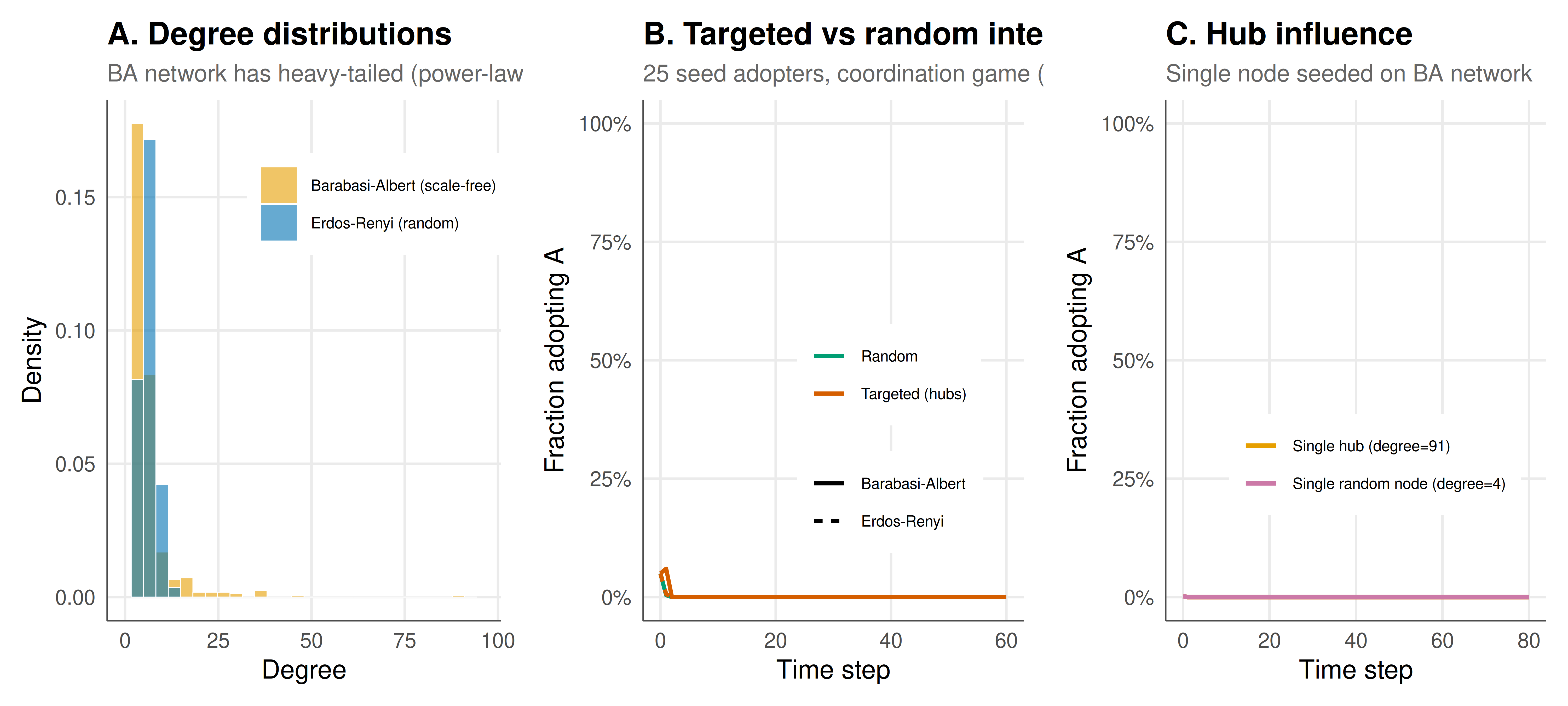
The figure presents three panels: degree distributions, adoption dynamics under different interventions, and the influence of a single hub versus a random node.
```{r}
#| label: fig-network-static
#| fig-cap: "Figure 1. Left: Degree distributions of Barabasi-Albert (scale-free) and Erdos-Renyi networks with 500 nodes and matched average degree. The BA network shows a heavy right tail characteristic of power-law distributions. Centre: Adoption of strategy A in a coordination game (a=3, b=2) with 25 seed nodes, comparing targeted (hub) vs random seeding on both network types. Right: Adoption cascade from seeding a single highest-degree hub versus a single random low-degree node on the BA network."
#| dev: [png, pdf]
#| fig-width: 10
#| fig-height: 4.5
#| dpi: 300
# Panel A: Degree distributions
p_deg <- ggplot(deg_dist, aes(x = degree, fill = network)) +
  geom_histogram(aes(y = after_stat(density)),
                 bins = 30, alpha = 0.6, position = "identity",
                 colour = "white", linewidth = 0.2) +
  scale_fill_manual(values = okabe_ito[c(1, 5)]) +
  scale_x_continuous(limits = c(0, max(deg_ba) + 5)) +
  labs(
    title = "A. Degree distributions",
    subtitle = "BA network has heavy-tailed (power-law) distribution",
    x = "Degree", y = "Density", fill = NULL
  ) +
  theme_publication() +
  theme(legend.position = c(0.7, 0.8),
        legend.background = element_rect(fill = "white", colour = NA),
        legend.text = element_text(size = 7))

# Panel B: Intervention comparison
p_adopt <- ggplot(sim_all,
       aes(x = time, y = frac_A, colour = intervention, linetype = network)) +
  geom_line(linewidth = 0.9) +
  scale_colour_manual(values = okabe_ito[c(3, 6)]) +
  scale_y_continuous(labels = scales::percent_format(), limits = c(0, 1)) +
  labs(
    title = "B. Targeted vs random intervention",
    subtitle = "25 seed adopters, coordination game (a=3, b=2)",
    x = "Time step", y = "Fraction adopting A",
    colour = NULL, linetype = NULL
  ) +
  theme_publication() +
  theme(legend.position = c(0.65, 0.35),
        legend.background = element_rect(fill = "white", colour = NA),
        legend.text = element_text(size = 7))

# Panel C: Single hub vs random
p_single <- ggplot(single_compare, aes(x = time, y = frac_A, colour = label)) +
  geom_line(linewidth = 1) +
  scale_colour_manual(values = okabe_ito[c(1, 7)]) +
  scale_y_continuous(labels = scales::percent_format(), limits = c(0, 1)) +
  labs(
    title = "C. Hub influence",
    subtitle = "Single node seeded on BA network",
    x = "Time step", y = "Fraction adopting A",
    colour = NULL
  ) +
  theme_publication() +
  theme(legend.position = c(0.55, 0.3),
        legend.background = element_rect(fill = "white", colour = NA),
        legend.text = element_text(size = 7))

gridExtra::grid.arrange(p_deg, p_adopt, p_single, ncol = 3)
```
## Interactive figure
Explore the adoption dynamics interactively. Hover over the curves to see the exact adoption fraction at each time step, and compare the four intervention scenarios.
```{r}
#| label: fig-network-interactive
p_int <- ggplot(sim_all,
       aes(x = time, y = frac_A, colour = interaction(intervention, network),
           text = paste0("Network: ", network,
                         "\nIntervention: ", intervention,
                         "\nTime: ", time,
                         "\nAdoption: ", round(frac_A, 3)))) +
  geom_line(linewidth = 0.8) +
  scale_colour_manual(
    values = okabe_ito[c(1, 3, 5, 6)],
    labels = c("BA + Random", "BA + Targeted",
               "ER + Random", "ER + Targeted")
  ) +
  scale_y_continuous(labels = scales::percent_format()) +
  labs(
    title = "Coordination game adoption dynamics: targeted vs random seeding",
    x = "Time step", y = "Fraction adopting strategy A",
    colour = NULL
  ) +
  theme_publication()

ggplotly(p_int, tooltip = "text") %>%
  config(displaylogo = FALSE) %>%
  layout(legend = list(orientation = "h", y = -0.2))
```
## Interpretation
The results confirm the theoretical prediction that network topology fundamentally shapes strategic outcomes. Three key findings emerge from the simulations.
First, **degree heterogeneity amplifies the effectiveness of targeted interventions**. On the Barabasi-Albert network, seeding the 25 highest-degree nodes produces dramatically faster adoption of strategy A compared to seeding 25 random nodes. The gap is much smaller on the Erdos-Renyi network, where degree homogeneity means that "high-degree" nodes are not much more influential than average nodes. This asymmetry is a direct consequence of the power-law degree distribution: in the BA network, the top 5% of nodes by degree account for a disproportionate share of all edges, so converting them influences a large fraction of the network immediately.
Second, **hubs act as equilibrium selectors**. The single-hub experiment shows that seeding just one highly connected node can trigger a cascade that eventually converts a substantial portion of the network. A single peripheral node, by contrast, may fail to trigger any cascade at all, because its few neighbours do not reach the adoption threshold. This has profound implications for equilibrium selection theory: in a multiplicity-of-equilibria setting, the initial strategic choices of hub nodes can determine which equilibrium the entire network converges to.
Third, **the coordination threshold interacts with network structure**. The threshold $q^* = b/(a+b)$ determines how many of a node's neighbours must adopt A before the node switches. On a scale-free network, hubs are the first to switch (they have the most seeded neighbours), and their switching immediately pushes many additional nodes past the threshold. This creates a snowball effect that is absent in homogeneous networks.
These findings have direct policy relevance. In epidemiology, the "vaccinate the hubs" strategy is known to be far more effective than random vaccination for controlling disease spread on scale-free networks [@nowak_may_1992]. In technology adoption, identifying and converting influential early adopters (the hubs of a social network) can determine whether a new standard achieves critical mass. In online platform competition, the users with the most connections serve as de facto kingmakers in the coordination game of platform choice.
## Extensions & related tutorials
The interplay between network structure and strategic behaviour is a rich research frontier. The techniques introduced here extend naturally to richer game structures, dynamic network formation, and empirical network data.
- [Diffusion cascades on networks](../../network-science/diffusion-cascades-networks/) --- detailed analysis of cascade dynamics and tipping points, building on the coordination game framework developed here
- [Centrality measures in game theory](../../network-science/centrality-measures-game-theory/) --- how different notions of centrality (degree, betweenness, eigenvector) predict strategic influence
- [Voting paradoxes and strategic voting](../../ethics-and-game-theory/voting-paradoxes-strategic/) --- strategic behaviour in a different collective-action setting, with connections to network-based opinion formation
- [Interactive game theory dashboards](../../visualization-and-communication/interactive-game-theory-dashboards/) --- advanced plotly techniques for visualising the network dynamics shown here
## References
::: {#refs}
:::