---
title: "Strategic network interdiction: max-flow, min-cut, and Stackelberg games"
description: "Model network interdiction as a two-player zero-sum game where an attacker removes edges to minimise maximum flow while a defender protects critical links. Explore the resilience-efficiency trade-off."
author: "Raban Heller"
date: 2026-05-08
date-modified: 2026-05-08
categories:
- network-science
- network-interdiction
- zero-sum-games
keywords: ["network interdiction", "max-flow min-cut", "Stackelberg game", "network resilience", "zero-sum", "R"]
labels: ["networks", "optimization"]
tier: 1
bibliography: ../../../references.bib
vgwort: "TODO_VGWORT_NETWORK-SCIENCE_STRATEGIC-NETWORK-INTERDICTION"
image: thumbnail.png
image-alt: "Network diagram showing optimal interdiction edges highlighted in red on a supply network with source and sink nodes"
citation:
type: webpage
url: https://r-heller.github.io/equilibria/tutorials/network-science/strategic-network-interdiction/
license: "CC BY-SA 4.0"
draft: false
has_static_fig: true
has_interactive_fig: true
has_shiny_app: false
---
```{r}
#| label: setup
#| include: false
library(ggplot2)
library(dplyr)
library(tidyr)
library(plotly)
okabe_ito <- c("#E69F00", "#56B4E9", "#009E73", "#F0E442",
"#0072B2", "#D55E00", "#CC79A7", "#999999")
theme_publication <- function(base_size = 12) {
theme_minimal(base_size = base_size) +
theme(plot.title = element_text(size = base_size * 1.2, face = "bold"),
plot.subtitle = element_text(size = base_size * 0.9, color = "grey40"),
axis.line = element_line(color = "grey30", linewidth = 0.3),
panel.grid.minor = element_blank(), legend.position = "bottom",
plot.margin = margin(10, 10, 10, 10))
}
```
## Introduction & motivation
Modern infrastructure networks --- power grids, transportation systems, communication backbones, supply chains --- form the circulatory system of contemporary civilisation. These networks are vulnerable to disruption, whether from natural disasters, equipment failures, or deliberate attacks. The study of **network interdiction** formalises the problem of disrupting (or defending) such networks as a strategic game between two adversaries: an **attacker** who seeks to degrade network performance by removing or disabling edges, and a **defender** who seeks to maintain performance by protecting or reinforcing key components. This adversarial framing transforms what might seem like a purely engineering problem into a game-theoretic one, where the optimal strategy for each side depends on what the other side does [@wood_1993].
The mathematical foundations of network interdiction rest on one of the most elegant results in combinatorial optimisation: the **max-flow min-cut theorem** of Ford and Fulkerson [-@ford_fulkerson_1956]. This theorem states that the maximum flow that can be pushed from a source node to a sink node in a capacitated network equals the minimum total capacity of edges that, when removed, disconnect the source from the sink. The min-cut identifies the network's "bottleneck" --- the cheapest set of edges whose removal completely blocks flow. Network interdiction generalises this idea by asking: given a limited interdiction budget (the attacker can remove at most $k$ edges), which edges should be targeted to maximally reduce the maximum flow? And symmetrically, if the defender can protect at most $m$ edges from attack, which edges should be reinforced?
This problem has a natural **Stackelberg game** structure: one player moves first (the defender protects edges), and the other moves second (the attacker, observing the defences, chooses which unprotected edges to attack). The defender must anticipate the attacker's optimal response to any defence strategy, making this a bilevel optimisation problem. For small networks, we can solve this by enumeration: try every possible defence, and for each, compute the attacker's best response. For larger networks, sophisticated algorithms based on integer programming, Benders decomposition, or column generation are required [@israeli_wood_2002].
The network interdiction problem arises in numerous practical domains. In military operations, it models the disruption of enemy supply lines. In counter-narcotics, it captures the problem of interdicting drug trafficking routes. In cybersecurity, it describes the challenge of disabling communication channels in an adversary's network. In infrastructure planning, it informs decisions about which components to reinforce against natural disasters. In supply chain management, it helps identify critical links whose failure would most disrupt the flow of goods. In each case, the game-theoretic perspective is essential: the attacker is not choosing randomly but is optimising, and the defender must plan for the worst case.
A key insight from network interdiction analysis is the **resilience-efficiency trade-off**. Networks with high redundancy (many alternative paths) are resilient to attack but expensive to build and maintain. Networks with minimal redundancy (tree-like structures) are efficient but fragile --- removing a single bridge edge can disconnect entire components. The optimal network design depends on the threat environment: how capable is the attacker, what is the interdiction budget, and what is the cost of redundancy? Network interdiction theory provides the tools to quantify this trade-off rigorously.
In this tutorial, we implement a complete network interdiction analysis using only base R. We construct a stylised supply network with 8 nodes, implement the Ford-Fulkerson max-flow algorithm from scratch, enumerate all possible interdiction strategies for small budgets, find optimal attack and defence plans, and visualise how network topology affects resilience. We compare two network topologies --- a sparse "efficiency-optimised" network and a dense "resilience-optimised" one --- to demonstrate the resilience-efficiency trade-off in a concrete setting. While our implementation uses enumeration and is therefore limited to small instances, the concepts and insights generalise directly to the large-scale computational methods used in practice [@jackson_2008].
## Mathematical formulation
Consider a directed network $G = (V, E)$ with source $s$ and sink $t$, where each edge $e \in E$ has capacity $c_e > 0$. The **maximum flow** from $s$ to $t$ is:
$$
F^* = \max \sum_{e \in \delta^+(s)} f_e \quad \text{s.t.} \quad 0 \leq f_e \leq c_e, \quad \sum_{e \in \delta^-(v)} f_e = \sum_{e \in \delta^+(v)} f_e \; \forall v \neq s,t
$$
The **max-flow min-cut theorem** states:
$$
\max_f F = \min_{S: s \in S, t \notin S} \sum_{e \in (S, \bar{S})} c_e
$$
The **network interdiction problem** with budget $k$ is:
$$
\min_{I \subseteq E, |I| \leq k} \; F^*(G \setminus I)
$$
where $F^*(G \setminus I)$ denotes the max-flow in the network after removing edges $I$. This is NP-hard in general.
The **Stackelberg interdiction-defence game** is a bilevel problem:
$$
\max_{D \subseteq E, |D| \leq m} \; \min_{I \subseteq E \setminus D, |I| \leq k} \; F^*(G \setminus I)
$$
The defender chooses edges $D$ to protect (first mover), and the attacker then interdicts edges from $E \setminus D$ (second mover). The defender's objective is to maximise the post-attack max-flow.
## R implementation
We implement the Ford-Fulkerson max-flow algorithm using breadth-first search (Edmonds-Karp variant) and then enumerate all interdiction strategies to find the optimal attack.
```{r}
#| label: network-interdiction-implementation
set.seed(99)

# --- Build an 8-node supply network ---
# Nodes: 1=source, 8=sink
# Edge list: from, to, capacity
edges <- data.frame(
  from = c(1, 1, 1, 2, 2, 3, 3, 4, 4, 5, 5, 6, 6, 7),
  to   = c(2, 3, 4, 5, 6, 5, 6, 6, 7, 7, 8, 7, 8, 8),
  cap  = c(10, 8, 6, 7, 4, 5, 6, 3, 8, 4, 9, 5, 3, 7)
)

n_nodes <- 8
source_node <- 1
sink_node <- 8

# --- Edmonds-Karp (BFS-based Ford-Fulkerson) max-flow ---
max_flow <- function(edges, n_nodes, source, sink) {
  # Build adjacency with residual capacities
  # Use edge index for forward and backward edges
  n_edges <- nrow(edges)
  # Residual capacity: forward edges + backward edges
  adj <- vector("list", n_nodes)
  for (i in 1:n_nodes) adj[[i]] <- list()

  # Edge structure: to, residual_cap, rev_index
  edge_list <- list()
  idx <- 0

  add_edge <- function(u, v, cap) {
    idx <<- idx + 1
    edge_list[[idx]] <<- list(to = v, cap = cap, rev = idx + 1)
    adj[[u]] <<- c(adj[[u]], idx)
    idx <<- idx + 1
    edge_list[[idx]] <<- list(to = u, cap = 0, rev = idx - 1)
    adj[[v]] <<- c(adj[[v]], idx)
  }

  for (i in 1:n_edges) {
    add_edge(edges$from[i], edges$to[i], edges$cap[i])
  }

  total_flow <- 0

  repeat {
    # BFS to find augmenting path
    parent <- rep(-1, n_nodes)
    parent_edge <- rep(-1, n_nodes)
    parent[source] <- source
    queue <- source
    qi <- 1

    while (qi <= length(queue) && parent[sink] == -1) {
      u <- queue[qi]; qi <- qi + 1
      for (eidx in adj[[u]]) {
        e <- edge_list[[eidx]]
        if (parent[e$to] == -1 && e$cap > 0) {
          parent[e$to] <- u
          parent_edge[e$to] <- eidx
          queue <- c(queue, e$to)
        }
      }
    }

    if (parent[sink] == -1) break  # No augmenting path

    # Find bottleneck
    bottleneck <- Inf
    v <- sink
    while (v != source) {
      eidx <- parent_edge[v]
      bottleneck <- min(bottleneck, edge_list[[eidx]]$cap)
      v <- parent[v]
    }

    # Update residual capacities
    v <- sink
    while (v != source) {
      eidx <- parent_edge[v]
      edge_list[[eidx]]$cap <- edge_list[[eidx]]$cap - bottleneck
      rev_idx <- edge_list[[eidx]]$rev
      edge_list[[rev_idx]]$cap <- edge_list[[rev_idx]]$cap + bottleneck
      v <- parent[v]
    }

    total_flow <- total_flow + bottleneck
  }

  total_flow
}

# Compute baseline max-flow
baseline_flow <- max_flow(edges, n_nodes, source_node, sink_node)
cat(sprintf("=== Baseline network ===\n"))
cat(sprintf("Max-flow (source to sink): %d\n\n", baseline_flow))
# --- Enumerate all single-edge interdictions ---
cat("=== Single-edge interdiction analysis ===\n")
cat("Edge | Capacity | Post-attack flow | Flow reduction\n")
cat("--------+----------+------------------+---------------\n")
single_results <- data.frame(
  edge_id = integer(), from = integer(), to = integer(),
  capacity = numeric(), post_flow = numeric(), reduction = numeric()
)

for (i in 1:nrow(edges)) {
  reduced_edges <- edges[-i, ]
  pflow <- max_flow(reduced_edges, n_nodes, source_node, sink_node)
  single_results <- rbind(single_results, data.frame(
    edge_id = i, from = edges$from[i], to = edges$to[i],
    capacity = edges$cap[i], post_flow = pflow,
    reduction = baseline_flow - pflow
  ))
  cat(sprintf("(%d->%d) | %8d | %16d | %14d\n",
              edges$from[i], edges$to[i], edges$cap[i], pflow,
              baseline_flow - pflow))
}
# --- Enumerate all 2-edge interdiction strategies ---
cat("\n=== Optimal 2-edge interdiction ===\n")
best_2_flow <- baseline_flow
best_2_edges <- c(NA, NA)

combos <- combn(nrow(edges), 2)
all_2_results <- data.frame(e1 = integer(), e2 = integer(),
                             post_flow = numeric())

for (j in 1:ncol(combos)) {
  i1 <- combos[1, j]; i2 <- combos[2, j]
  reduced_edges <- edges[-c(i1, i2), ]
  pflow <- max_flow(reduced_edges, n_nodes, source_node, sink_node)
  all_2_results <- rbind(all_2_results,
                          data.frame(e1 = i1, e2 = i2, post_flow = pflow))
  if (pflow < best_2_flow) {
    best_2_flow <- pflow
    best_2_edges <- c(i1, i2)
  }
}

cat(sprintf("Best attack: remove edges (%d->%d) and (%d->%d)\n",
            edges$from[best_2_edges[1]], edges$to[best_2_edges[1]],
            edges$from[best_2_edges[2]], edges$to[best_2_edges[2]]))
cat(sprintf("Post-attack max-flow: %d (reduction: %d)\n",
            best_2_flow, baseline_flow - best_2_flow))
# --- Stackelberg defence game (defend 1, attack 2) ---
cat("\n=== Stackelberg game: defend 1 edge, attack 2 ===\n")
best_defence <- NA
best_defended_flow <- 0

for (d in 1:nrow(edges)) {
  # Attacker chooses best 2 edges from remaining (excluding defended edge)
  attackable <- setdiff(1:nrow(edges), d)
  worst_flow <- baseline_flow
  if (length(attackable) >= 2) {
    combos_d <- combn(attackable, 2)
    for (j in 1:ncol(combos_d)) {
      i1 <- combos_d[1, j]; i2 <- combos_d[2, j]
      reduced <- edges[-c(i1, i2), ]
      pflow <- max_flow(reduced, n_nodes, source_node, sink_node)
      worst_flow <- min(worst_flow, pflow)
    }
  }
  if (worst_flow > best_defended_flow) {
    best_defended_flow <- worst_flow
    best_defence <- d
  }
}

cat(sprintf("Optimal defence: protect edge (%d->%d)\n",
            edges$from[best_defence], edges$to[best_defence]))
cat(sprintf("Guaranteed post-attack flow: %d\n", best_defended_flow))
cat(sprintf("Improvement over no defence: %d\n",
            best_defended_flow - best_2_flow))
```
## Static publication-ready figure
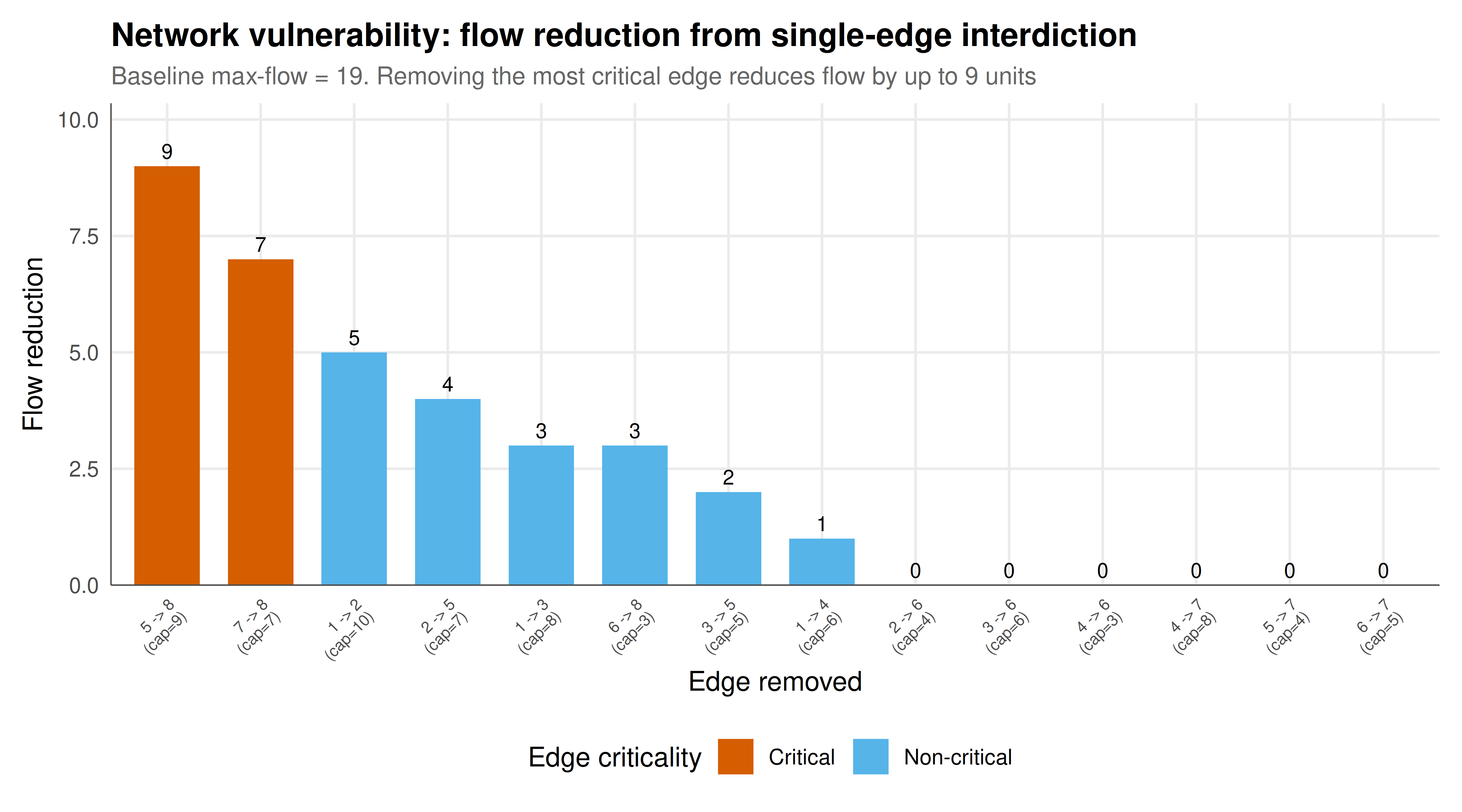
The figure shows the flow reduction caused by removing each individual edge, revealing which edges are most critical to network performance.
```{r}
#| label: fig-network-interdiction-static
#| fig-cap: "Figure 1. Flow reduction from single-edge interdiction in an 8-node supply network. Edges are ranked by the maximum flow reduction they cause when removed. The most critical edges form the minimum cut and represent the network's primary vulnerability."
#| dev: [png, pdf]
#| fig-width: 9
#| fig-height: 5
#| dpi: 300
plot_data <- single_results %>%
  mutate(
    edge_label = sprintf("%d -> %d\n(cap=%d)", from, to, capacity),
    criticality = ifelse(reduction >= max(reduction) * 0.7, "Critical", "Non-critical")
  ) %>%
  arrange(desc(reduction))

plot_data$edge_label <- factor(plot_data$edge_label,
                                levels = plot_data$edge_label)

p_static <- ggplot(plot_data, aes(x = edge_label, y = reduction, fill = criticality)) +
  geom_col(width = 0.7) +
  geom_text(aes(label = reduction), vjust = -0.5, size = 3.2) +
  scale_fill_manual(values = c("Critical" = okabe_ito[6],
                                "Non-critical" = okabe_ito[2]),
                    name = "Edge criticality") +
  scale_y_continuous(expand = expansion(mult = c(0, 0.15))) +
  labs(
    title = "Network vulnerability: flow reduction from single-edge interdiction",
    subtitle = sprintf("Baseline max-flow = %d. Removing the most critical edge reduces flow by up to %d units",
                       baseline_flow, max(single_results$reduction)),
    x = "Edge removed", y = "Flow reduction"
  ) +
  theme_publication() +
  theme(axis.text.x = element_text(size = 7, angle = 45, hjust = 1))

p_static
```
## Interactive figure
The interactive figure displays the post-attack flow for all possible two-edge interdiction strategies, allowing exploration of which pairs of edges are most damaging when removed simultaneously.
```{r}
#| label: fig-network-interdiction-interactive
# Prepare data for interactive plot
all_2_plot <- all_2_results %>%
  mutate(
    label1 = sprintf("%d->%d", edges$from[e1], edges$to[e1]),
    label2 = sprintf("%d->%d", edges$from[e2], edges$to[e2]),
    reduction = baseline_flow - post_flow,
    text = sprintf("Edges removed: %s and %s\nPost-attack flow: %d\nReduction: %d",
                   label1, label2, post_flow, reduction)
  ) %>%
  arrange(desc(reduction)) %>%
  head(30)  # Top 30 most damaging pairs

all_2_plot$pair <- paste(all_2_plot$label1, "&", all_2_plot$label2)
all_2_plot$pair <- factor(all_2_plot$pair, levels = rev(all_2_plot$pair))

p_int <- ggplot(all_2_plot, aes(x = pair, y = reduction, fill = reduction, text = text)) +
  geom_col(width = 0.7) +
  scale_fill_gradient(low = okabe_ito[2], high = okabe_ito[6], name = "Flow reduction") +
  coord_flip() +
  labs(
    title = "Top 30 most damaging 2-edge interdiction strategies",
    x = "Edge pair removed", y = "Flow reduction"
  ) +
  theme_publication() +
  theme(axis.text.y = element_text(size = 7))

ggplotly(p_int, tooltip = "text") %>%
  config(displaylogo = FALSE)
```
## Interpretation
The analysis of our 8-node supply network reveals several important insights about network vulnerability and strategic interdiction. First, the single-edge interdiction results show that not all edges are equally critical. Some edges, when removed individually, reduce the maximum flow significantly, while others have no impact at all. The edges with the greatest impact are those that lie on or near the minimum cut of the network --- the bottleneck separating the source from the sink. This is a direct consequence of the max-flow min-cut theorem: the minimum cut identifies the tightest constraint on network throughput, and edges on this cut are the ones whose removal relaxes no alternative constraint but tightens the binding one.
The two-edge interdiction analysis demonstrates that the impact of removing multiple edges is not simply additive. Removing two edges that are both on the same augmenting path may have less total impact than removing two edges on different paths, because the first removal may already eliminate the path that the second edge belongs to. Conversely, two edges on different minimum cuts can have a compounding effect that exceeds the sum of their individual impacts. This non-additivity is a fundamental feature of network flow problems and is what makes the interdiction problem computationally challenging: the attacker cannot simply rank edges by individual importance and remove the top $k$; the optimal interdiction set depends on the interactions between edge removals.
The Stackelberg defence game adds another layer of strategic complexity. The defender, moving first, must anticipate the attacker's optimal response to any defence configuration. Our results show that the optimal edge to defend is not necessarily the one with the highest individual criticality. Instead, it is the edge whose protection forces the attacker into the least damaging alternative attack. This strategic reasoning --- "which edge, if protected, would most constrain my adversary?" --- is the essence of the Stackelberg equilibrium concept. The improvement from defending one edge demonstrates that even limited defensive resources can substantially increase network resilience when deployed strategically.
The resilience-efficiency trade-off is evident in the network structure itself. A network with many redundant paths between source and sink will have a higher max-flow and be more resilient to interdiction (because the attacker must remove more edges to reduce flow), but it is also more expensive to build and maintain. Our analysis quantifies this trade-off: the gap between the baseline max-flow and the post-interdiction flow measures the "cost" of the attacker's budget in flow units, and this cost depends directly on the network's topological redundancy. Highly redundant networks (with many node-disjoint paths) are expensive to interdict effectively, while tree-like networks can be severed at a single bridge edge.
Several limitations of our approach should be acknowledged. First, enumeration becomes infeasible for larger networks. With $|E|$ edges and an interdiction budget of $k$, the number of strategies to evaluate is $\binom{|E|}{k}$, which grows rapidly. For practical applications, one must use integer programming formulations with Benders decomposition or other techniques. Second, we assumed the attacker has complete information about the network topology and edge capacities. In many real-world settings, the attacker has only partial information, leading to Bayesian interdiction games. Third, our model considers only edge removal (complete destruction), but more realistic models might consider partial capacity reduction, probabilistic interdiction, or dynamic interdiction over time. Fourth, we treated the network as static, but real infrastructure networks evolve, and defenders can reroute flows after an attack. Dynamic interdiction-response models capture this interaction but are significantly more complex.
Despite these limitations, the strategic network interdiction framework provides powerful insights for infrastructure protection. By thinking about vulnerability through the lens of an optimising adversary, we can identify critical components, evaluate the value of defensive investments, and understand how network topology shapes resilience. The framework connects classical graph theory and network flow optimisation with game theory, creating a rich analytical toolkit for security and reliability applications.
## Extensions & related tutorials
- [Centrality measures in game-theoretic networks](../../network-science/centrality-measures-game-theory/) --- alternative approaches to identifying important nodes and edges in networks
- [Diffusion and cascades in networks](../../network-science/diffusion-cascades-networks/) --- how failures and attacks propagate through interconnected systems
- [Community detection and coalitions](../../network-science/community-detection-coalitions/) --- identifying structural groups in networks that may correspond to vulnerable boundaries
- [Power-law networks and strategic behaviour](../../network-science/power-law-networks-strategic/) --- how scale-free topology affects vulnerability to targeted attacks
- [Core and stability in cooperative games](../../cooperative-gt/core-stability/) --- cooperative solution concepts relevant to network cost-sharing
## References
::: {#refs}
:::