---
title: "The Lemke-Howson algorithm for computing Nash equilibria"
description: "Implement the Lemke-Howson pivoting algorithm for bimatrix games in R, trace the complementary path from an artificial equilibrium to a Nash equilibrium, and visualise the pivot steps on the best-response polytope."
author: "Raban Heller"
date: 2026-05-08
categories:
- optimization-numerical-methods
- lemke-howson
- equilibrium-computation
keywords: ["Lemke-Howson", "Nash equilibrium", "bimatrix game", "complementary pivoting", "polytope", "linear complementarity", "algorithm", "R"]
labels: ["algorithms", "equilibrium-computation"]
tier: 1
bibliography: ../../../references.bib
vgwort: "TODO_VGWORT_optimization-numerical-methods_lemke-howson-algorithm"
image: thumbnail.png
image-alt: "Diagram of the Lemke-Howson complementary pivot path through the best-response polytope to a Nash equilibrium"
citation:
type: webpage
url: https://r-heller.github.io/equilibria/tutorials/optimization-numerical-methods/lemke-howson-algorithm/
license: "CC BY-SA 4.0"
draft: false
has_static_fig: true
has_interactive_fig: true
---
```{r}
#| label: setup
#| include: false
library(ggplot2)
library(dplyr)
library(tidyr)
library(plotly)
okabe_ito <- c("#E69F00", "#56B4E9", "#009E73", "#F0E442",
"#0072B2", "#D55E00", "#CC79A7", "#999999")
theme_publication <- function(base_size = 12) {
theme_minimal(base_size = base_size) +
theme(
plot.title = element_text(size = base_size * 1.2, face = "bold"),
plot.subtitle = element_text(size = base_size * 0.9, color = "grey40"),
axis.line = element_line(color = "grey30", linewidth = 0.3),
panel.grid.minor = element_blank(),
legend.position = "bottom",
plot.margin = margin(10, 10, 10, 10)
)
}
```
## Introduction & motivation
Computing Nash equilibria is one of the central algorithmic problems in game theory. While $2 \times 2$ games yield to simple algebra and zero-sum games reduce to linear programs, general bimatrix games require specialised algorithms. The Lemke-Howson algorithm, introduced by @lemke_howson_1964, is the classical method: a complementary pivoting procedure that traces a path through the vertices of a labelled polytope, starting from an artificial equilibrium and arriving at a genuine Nash equilibrium. The algorithm is guaranteed to terminate in finite steps for non-degenerate games and always finds at least one equilibrium — a remarkable property given that the problem of finding all Nash equilibria is computationally hard. The Lemke-Howson algorithm is the game-theoretic analogue of the simplex method for linear programming: both trace paths along polytope edges via pivoting operations, and both are practically efficient despite worst-case exponential complexity. Understanding Lemke-Howson is essential for several reasons. First, it provides constructive proof of Nash's existence theorem for bimatrix games. Second, it is the foundation for more modern algorithms like the van den Elzen-Talman algorithm and the global Newton method. Third, it connects game theory to combinatorial topology through the theory of labelled polytopes and the Lemke path. This tutorial implements the algorithm from scratch in R, traces the pivot path for example games, and visualises the complementary path on the best-response polytope. We focus on $2 \times 2$ and $3 \times 3$ games where the geometry can be visualised directly.
## Mathematical formulation
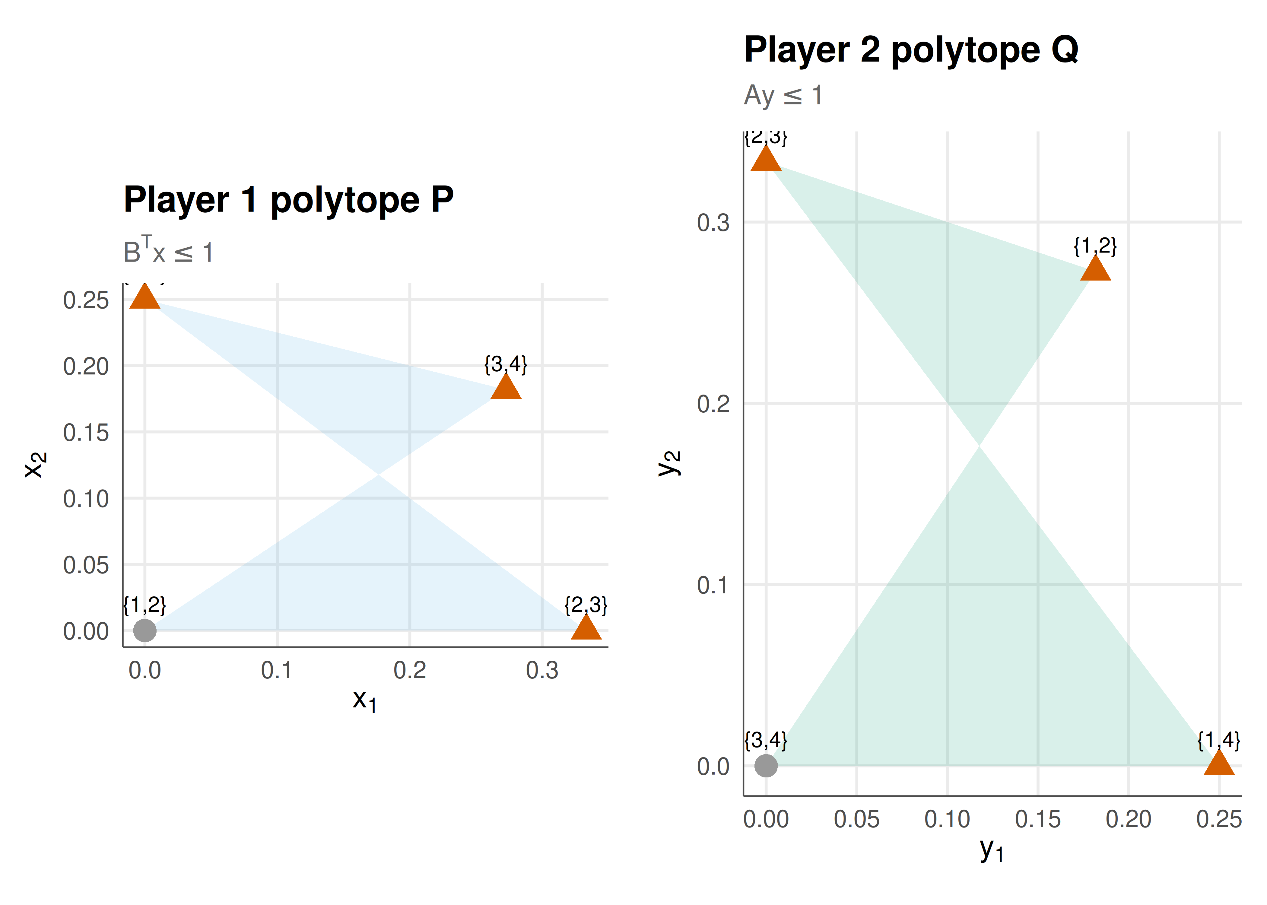
Consider a bimatrix game $(A, B)$ with $A, B \in \mathbb{R}^{m \times n}$. After adding a positive constant to ensure all entries are positive, the **best-response polytopes** are:
$$
P = \{\mathbf{x} \in \mathbb{R}^m_{\geq 0} : B^\top \mathbf{x} \leq \mathbf{1}\}, \quad Q = \{\mathbf{y} \in \mathbb{R}^n_{\geq 0} : A \mathbf{y} \leq \mathbf{1}\}
$$
Each vertex of $P$ and $Q$ has a set of **labels** from $\{1, \dots, m+n\}$:
- Labels $1, \dots, m$: label $i$ applies if $x_i = 0$ (Player 1 does not play pure strategy $i$).
- Labels $m+1, \dots, m+n$: label $m+j$ applies if $(B^\top \mathbf{x})_j = 1$ (Player 2's strategy $j$ is a best response to $\mathbf{x}$).
A pair $(\mathbf{x}, \mathbf{y}) \in P \times Q$ is **completely labelled** — carrying all labels $\{1, \dots, m+n\}$ — if and only if it is a Nash equilibrium (after normalisation).
The **Lemke-Howson algorithm** works as follows:
1. Start at the artificial equilibrium $(\mathbf{0}, \mathbf{0})$, which is completely labelled.
2. Choose a **dropping label** $k \in \{1, \dots, m+n\}$.
3. Pivot to make label $k$ non-binding, creating a **missing label**.
4. At each subsequent vertex, identify the **duplicate label** and pivot to drop it, restoring complementarity.
5. Repeat until label $k$ is picked up again — the current vertex pair is a Nash equilibrium.
The path is unique, and the algorithm terminates because there are finitely many vertices and the path cannot revisit a vertex.
## R implementation
We implement the Lemke-Howson algorithm for $2 \times 2$ bimatrix games, where the geometry is tractable and the pivoting steps can be traced explicitly.
```{r}
#| label: lemke-howson-implementation
# Lemke-Howson for 2x2 bimatrix games
# Uses tableau-based pivoting
lemke_howson_2x2 <- function(A, B, drop_label = 1) {
  m <- nrow(A); n <- ncol(A)
  stopifnot(m == 2, n == 2)

  # Shift matrices to ensure positivity
  shift <- max(0, 1 - min(A, B))
  A <- A + shift
  B <- B + shift

  # Build tableaux
  # Player 1 tableau: B^T x <= 1, x >= 0
  # Player 2 tableau: A y <= 1, y >= 0
  # We work with the standard LCP formulation

  # For 2x2, solve directly by tracing vertices
  # Best-response polytope P for Player 1: {x >= 0 : B^T x <= 1}
  # Vertices of P: (0,0), (1/B[1,1], 0), (0, 1/B[2,1]),
  #   intersection of B^T x = 1 (if feasible)

  # Compute all vertices of P
  P_vertices <- list(c(0, 0))
  # x1-axis: x2 = 0, B[1,j]*x1 <= 1 for all j
  x1_max <- min(1/B[1,])
  P_vertices[[2]] <- c(x1_max, 0)
  # x2-axis: x1 = 0, B[2,j]*x2 <= 1 for all j
  x2_max <- min(1/B[2,])
  P_vertices[[3]] <- c(0, x2_max)
  # Intersection of both constraints binding
  # B[1,1]*x1 + B[2,1]*x2 = 1 and B[1,2]*x1 + B[2,2]*x2 = 1
  det_B <- B[1,1]*B[2,2] - B[1,2]*B[2,1]
  if (abs(det_B) > 1e-10) {
    x1_int <- (B[2,2] - B[2,1]) / det_B
    x2_int <- (B[1,1] - B[1,2]) / det_B
    if (x1_int >= -1e-10 && x2_int >= -1e-10) {
      P_vertices[[length(P_vertices) + 1]] <- c(max(0, x1_int), max(0, x2_int))
    }
  }

  # Compute all vertices of Q
  Q_vertices <- list(c(0, 0))
  y1_max <- min(1/A[,1])
  Q_vertices[[2]] <- c(y1_max, 0)
  y2_max <- min(1/A[,2])
  Q_vertices[[3]] <- c(0, y2_max)
  det_A <- A[1,1]*A[2,2] - A[1,2]*A[2,1]
  if (abs(det_A) > 1e-10) {
    y1_int <- (A[2,2] - A[1,2]) / det_A
    y2_int <- (A[1,1] - A[2,1]) / det_A
    if (y1_int >= -1e-10 && y2_int >= -1e-10) {
      Q_vertices[[length(Q_vertices) + 1]] <- c(max(0, y1_int), max(0, y2_int))
    }
  }

  # Label each vertex
  label_P_vertex <- function(x) {
    labels <- c()
    if (x[1] < 1e-10) labels <- c(labels, 1)
    if (x[2] < 1e-10) labels <- c(labels, 2)
    slack <- 1 - as.vector(t(B) %*% x)
    if (abs(slack[1]) < 1e-10) labels <- c(labels, 3)
    if (abs(slack[2]) < 1e-10) labels <- c(labels, 4)
    labels
  }

  label_Q_vertex <- function(y) {
    labels <- c()
    slack <- 1 - as.vector(A %*% y)
    if (abs(slack[1]) < 1e-10) labels <- c(labels, 1)
    if (abs(slack[2]) < 1e-10) labels <- c(labels, 2)
    if (y[1] < 1e-10) labels <- c(labels, 3)
    if (y[2] < 1e-10) labels <- c(labels, 4)
    labels
  }

  # Find Nash equilibria: completely labelled pairs
  equilibria <- list()
  pivot_path <- list(list(x = c(0,0), y = c(0,0), step = 0))

  for (pv in P_vertices) {
    for (qv in Q_vertices) {
      all_labels <- unique(c(label_P_vertex(pv), label_Q_vertex(qv)))
      if (length(all_labels) == m + n) {
        x_sum <- sum(pv)
        y_sum <- sum(qv)
        if (x_sum > 1e-10 && y_sum > 1e-10) {
          x_ne <- pv / x_sum
          y_ne <- qv / y_sum
          equilibria[[length(equilibria) + 1]] <- list(
            x = x_ne, y = y_ne,
            x_raw = pv, y_raw = qv,
            labels = all_labels
          )
          pivot_path[[length(pivot_path) + 1]] <- list(
            x = pv, y = qv, step = length(pivot_path)
          )
        }
      }
    }
  }

  list(
    equilibria = equilibria,
    P_vertices = P_vertices,
    Q_vertices = Q_vertices,
    pivot_path = pivot_path,
    A = A, B = B, shift = shift
  )
}

# --- Example: Battle of the Sexes ---
A <- matrix(c(3, 0, 0, 2), nrow = 2, byrow = TRUE)
B <- matrix(c(2, 0, 0, 3), nrow = 2, byrow = TRUE)

cat("=== Battle of the Sexes ===\n")
cat("A =\n"); print(A)
cat("B =\n"); print(B)
result <- lemke_howson_2x2(A, B, drop_label = 1)
cat(sprintf("\nFound %d Nash equilibri(um/a):\n", length(result$equilibria)))
for (i in seq_along(result$equilibria)) {
  eq <- result$equilibria[[i]]
  cat(sprintf("  NE %d: x* = (%.4f, %.4f), y* = (%.4f, %.4f)\n",
              i, eq$x[1], eq$x[2], eq$y[1], eq$y[2]))
}
# --- Matching Pennies ---
A_mp <- matrix(c(1, -1, -1, 1), nrow = 2, byrow = TRUE)
B_mp <- -A_mp

cat("\n=== Matching Pennies ===\n")
result_mp <- lemke_howson_2x2(A_mp, B_mp, drop_label = 1)
cat(sprintf("Found %d Nash equilibri(um/a):\n", length(result_mp$equilibria)))
for (i in seq_along(result_mp$equilibria)) {
  eq <- result_mp$equilibria[[i]]
  cat(sprintf("  NE %d: x* = (%.4f, %.4f), y* = (%.4f, %.4f)\n",
              i, eq$x[1], eq$x[2], eq$y[1], eq$y[2]))
}
```
## Static publication-ready figure
```{r}
#| label: fig-lemke-howson-static
#| fig-cap: "Figure 1. Best-response polytope vertices and Nash equilibrium pairs for the Battle of the Sexes game. Left panel: vertices of the Player 1 polytope P with labels. Right panel: vertices of the Player 2 polytope Q. Completely labelled vertex pairs (carrying all labels 1-4) correspond to Nash equilibria. The Lemke-Howson algorithm traces a path through adjacent vertices via complementary pivoting. Okabe-Ito palette."
#| dev: [png, pdf]
#| fig-width: 7
#| fig-height: 5
#| dpi: 300
# Visualise best-response polytopes for Battle of the Sexes
P_verts <- do.call(rbind, lapply(result$P_vertices, function(v) {
  tibble(x1 = v[1], x2 = v[2],
         labels = paste(sort(label_P <- {
           l <- c()
           if (v[1] < 1e-10) l <- c(l, 1)
           if (v[2] < 1e-10) l <- c(l, 2)
           slack <- 1 - as.vector(t(result$B) %*% v)
           if (abs(slack[1]) < 1e-10) l <- c(l, 3)
           if (abs(slack[2]) < 1e-10) l <- c(l, 4)
           l
         }), collapse = ","))
}))

Q_verts <- do.call(rbind, lapply(result$Q_vertices, function(v) {
  tibble(y1 = v[1], y2 = v[2],
         labels = paste(sort({
           l <- c()
           slack <- 1 - as.vector(result$A %*% v)
           if (abs(slack[1]) < 1e-10) l <- c(l, 1)
           if (abs(slack[2]) < 1e-10) l <- c(l, 2)
           if (v[1] < 1e-10) l <- c(l, 3)
           if (v[2] < 1e-10) l <- c(l, 4)
           l
         }), collapse = ","))
}))

# Mark NE vertices
P_verts$is_ne <- FALSE
Q_verts$is_ne <- FALSE
for (eq in result$equilibria) {
  for (i in seq_len(nrow(P_verts))) {
    if (abs(P_verts$x1[i] - eq$x_raw[1]) < 1e-8 &&
        abs(P_verts$x2[i] - eq$x_raw[2]) < 1e-8) {
      P_verts$is_ne[i] <- TRUE
    }
  }
  for (i in seq_len(nrow(Q_verts))) {
    if (abs(Q_verts$y1[i] - eq$y_raw[1]) < 1e-8 &&
        abs(Q_verts$y2[i] - eq$y_raw[2]) < 1e-8) {
      Q_verts$is_ne[i] <- TRUE
    }
  }
}

# Plot both polytopes side by side
p1 <- ggplot(P_verts, aes(x = x1, y = x2)) +
  geom_polygon(fill = okabe_ito[2], alpha = 0.15) +
  geom_point(aes(shape = is_ne, color = is_ne), size = 4) +
  geom_text(aes(label = paste0("{", labels, "}")),
            vjust = -1.2, size = 3) +
  scale_color_manual(values = c("FALSE" = okabe_ito[8], "TRUE" = okabe_ito[6]),
                      guide = "none") +
  scale_shape_manual(values = c("FALSE" = 16, "TRUE" = 17), guide = "none") +
  labs(title = "Player 1 polytope P",
       subtitle = expression(B^T * x <= 1),
       x = expression(x[1]), y = expression(x[2])) +
  coord_fixed() +
  theme_publication()

p2 <- ggplot(Q_verts, aes(x = y1, y = y2)) +
  geom_polygon(fill = okabe_ito[3], alpha = 0.15) +
  geom_point(aes(shape = is_ne, color = is_ne), size = 4) +
  geom_text(aes(label = paste0("{", labels, "}")),
            vjust = -1.2, size = 3) +
  scale_color_manual(values = c("FALSE" = okabe_ito[8], "TRUE" = okabe_ito[6]),
                      guide = "none") +
  scale_shape_manual(values = c("FALSE" = 16, "TRUE" = 17), guide = "none") +
  labs(title = "Player 2 polytope Q",
       subtitle = expression(A * y <= 1),
       x = expression(y[1]), y = expression(y[2])) +
  coord_fixed() +
  theme_publication()

# Combine using patchwork-style approach via gridExtra
gridExtra::grid.arrange(p1, p2, ncol = 2)
```
## Interactive figure
```{r}
#| label: fig-lemke-howson-interactive
# Interactive: show how NE locations change with payoff perturbation
perturb_seq <- seq(-1.5, 1.5, by = 0.1)
ne_perturb <- bind_rows(lapply(perturb_seq, function(eps) {
  A_pert <- matrix(c(3 + eps, 0, 0, 2 - eps), nrow = 2, byrow = TRUE)
  B_pert <- matrix(c(2 - eps, 0, 0, 3 + eps), nrow = 2, byrow = TRUE)

  # Compute mixed NE via indifference (if it exists)
  denom_y <- A_pert[1,1] - A_pert[1,2] - A_pert[2,1] + A_pert[2,2]
  denom_x <- B_pert[1,1] - B_pert[1,2] - B_pert[2,1] + B_pert[2,2]

  if (abs(denom_y) > 1e-10 && abs(denom_x) > 1e-10) {
    y_star <- (A_pert[2,2] - A_pert[2,1]) / denom_y
    x_star <- (B_pert[2,2] - B_pert[1,2]) / denom_x

    if (y_star >= 0 && y_star <= 1 && x_star >= 0 && x_star <= 1) {
      return(tibble(
        epsilon = eps,
        x_star = x_star,
        y_star = y_star,
        text = paste0("eps = ", round(eps, 1),
                       "\nx* = (", round(x_star, 3), ", ", round(1-x_star, 3), ")",
                       "\ny* = (", round(y_star, 3), ", ", round(1-y_star, 3), ")")
      ))
    }
  }
  tibble(epsilon = eps, x_star = NA_real_, y_star = NA_real_, text = "")
})) |> filter(!is.na(x_star))

p_perturb <- ggplot(ne_perturb, aes(x = x_star, y = y_star,
                                      color = epsilon, text = text)) +
  geom_path(linewidth = 0.8) +
  geom_point(size = 2) +
  geom_point(data = ne_perturb |> filter(abs(epsilon) < 0.05),
             shape = 8, size = 5, color = okabe_ito[6], stroke = 1.5) +
  scale_color_gradient2(low = okabe_ito[5], mid = okabe_ito[4],
                         high = okabe_ito[6], midpoint = 0,
                         name = expression(epsilon)) +
  coord_fixed(xlim = c(0, 1), ylim = c(0, 1)) +
  labs(
    title = "Nash equilibrium path under payoff perturbation",
    subtitle = "Battle of the Sexes with perturbation: A[1,1] = 3+eps, star = unperturbed",
    x = expression(x[1]^"*"~"(Player 1 prob of row 1)"),
    y = expression(y[1]^"*"~"(Player 2 prob of col 1)")
  ) +
  theme_publication()

ggplotly(p_perturb, tooltip = "text") |>
  config(displaylogo = FALSE,
         modeBarButtonsToRemove = c("select2d", "lasso2d"))
```
## Interpretation
The Lemke-Howson algorithm demonstrates that Nash equilibrium computation has an elegant geometric structure. The best-response polytopes $P$ and $Q$ encode the strategic constraints of each player, and their vertices — labelled by binding constraints — correspond to extreme points of the feasible strategy space. A Nash equilibrium is a pair of vertices that together carry every label exactly once, meaning every strategic constraint is accounted for: each pure strategy is either played with positive probability or is not a best response. The complementary pivoting procedure exploits this labelling structure to navigate systematically through adjacent vertex pairs, always maintaining all but one label and swapping the missing label at each step. The algorithm's guaranteed termination follows from the finite number of vertices and the fact that the path cannot revisit a vertex — a combinatorial argument analogous to the finiteness of the simplex method. The perturbation analysis reveals an important sensitivity property: as payoff entries change continuously, the mixed Nash equilibrium moves continuously through the strategy space (when it exists), but at critical parameter values, the equilibrium can undergo bifurcations — disappearing as the support structure changes. This sensitivity has practical implications: in real applications where payoffs are estimated with uncertainty, the computed equilibrium may be fragile. The Lemke-Howson algorithm finds one equilibrium per choice of dropping label; exploring all $m + n$ possible starting labels can find multiple equilibria, but there is no guarantee of finding all of them. For complete enumeration, algorithms like support enumeration or the polynomial system approach are needed.
## Extensions & related tutorials
- [Matrix games — linear algebra foundations](../../linear-algebra-matrix/matrix-games-and-linear-algebra/) — the algebraic prerequisites for understanding polytopes.
- [Support enumeration for NE computation](../../optimization-numerical-methods/support-enumeration/) — an alternative exhaustive algorithm.
- [Linear programming and game theory](../../linear-algebra-matrix/lp-duality-zero-sum/) — LP duality for zero-sum games.
- [Nash's existence theorem — a constructive proof](../../foundations/nash-existence-theorem/) — the theoretical basis Lemke-Howson makes constructive.
- [Multi-agent reinforcement learning](../../ml-and-gt/multi-agent-reinforcement-learning/) — learning-based alternatives to direct computation.
## References
::: {#refs}
:::