---
title: "Support enumeration algorithm for Nash equilibria"
description: "Implement the support enumeration method to find all Nash equilibria of bimatrix games by solving indifference conditions for each support pair, with applications to games with multiple equilibria."
author: "Raban Heller"
date: 2026-05-08
date-modified: 2026-05-08
categories:
- optimization-numerical-methods
- nash-equilibrium
- support-enumeration
- bimatrix-games
keywords: ["support enumeration", "Nash equilibrium", "bimatrix games", "indifference conditions", "Lemke-Howson", "R"]
labels: ["optimization-numerical-methods", "nash-equilibrium"]
tier: 1
bibliography: ../../../references.bib
vgwort: "TODO_VGWORT_optimization-numerical-methods_support-enumeration-algorithm"
image: thumbnail.png
image-alt: "Scatter plot showing the support structure and probability weights of multiple Nash equilibria found by the support enumeration algorithm"
citation:
type: webpage
url: https://r-heller.github.io/equilibria/tutorials/optimization-numerical-methods/support-enumeration-algorithm/
license: "CC BY-SA 4.0"
draft: false
has_static_fig: true
has_interactive_fig: true
has_shiny_app: false
---
```{r}
#| label: setup
#| include: false
library(ggplot2)
library(dplyr)
library(tidyr)
library(plotly)
okabe_ito <- c("#E69F00", "#56B4E9", "#009E73", "#F0E442",
"#0072B2", "#D55E00", "#CC79A7", "#999999")
theme_publication <- function(base_size = 12) {
theme_minimal(base_size = base_size) +
theme(plot.title = element_text(size = base_size * 1.2, face = "bold"),
plot.subtitle = element_text(size = base_size * 0.9, color = "grey40"),
axis.line = element_line(color = "grey30", linewidth = 0.3),
panel.grid.minor = element_blank(), legend.position = "bottom",
plot.margin = margin(10, 10, 10, 10))
}
```
## Introduction & motivation
Finding Nash equilibria of bimatrix games is one of the central computational problems in game theory. While Nash's existence theorem [@nash_1950] guarantees that every finite game has at least one Nash equilibrium (possibly in mixed strategies), the theorem is non-constructive: it does not tell us how to find the equilibria or how many there are. For practical applications -- from analysing market competition to designing automated trading agents -- we need algorithms that can actually compute equilibria.
The **support enumeration algorithm** is the most conceptually transparent method for finding **all** Nash equilibria of a bimatrix game. The key insight is that a Nash equilibrium is characterised by two conditions: (1) every strategy played with positive probability (i.e., in the "support" of the equilibrium mixed strategy) must yield the same expected payoff against the opponent's mix, and (2) every strategy outside the support must yield a weakly lower payoff. The algorithm exploits this structure by systematically enumerating all possible pairs of supports (subsets of strategies for each player), solving the resulting linear system of indifference equations for each pair, and checking whether the solution satisfies the non-negativity and non-deviation conditions.
For a game where player 1 has $m$ strategies and player 2 has $n$ strategies, the number of possible support pairs is $\sum_{k=1}^{m} \binom{m}{k} \cdot \sum_{l=1}^{n} \binom{n}{l}$, which can be large but is manageable for small games. The algorithm's worst-case complexity is exponential in the game size, which is consistent with the PPAD-completeness of the general Nash equilibrium computation problem [@lemke_howson_1964]. However, for games up to about $4 \times 4$ or $5 \times 5$, the enumeration is perfectly tractable and has the major advantage of finding **all** equilibria, not just one.
This contrasts with the **Lemke-Howson algorithm** [@lemke_howson_1964], which is a complementary pivoting method (similar to the simplex method for LP) that efficiently finds a single Nash equilibrium but cannot easily enumerate all of them. The Lemke-Howson algorithm follows a path of "almost complementary" pairs of vertices in a labelled polytope, terminating at a Nash equilibrium. By starting from different initial pivots, one can sometimes find additional equilibria, but there is no guarantee of finding all of them without additional bookkeeping.
In this tutorial, we implement the support enumeration algorithm from scratch in R, apply it to several bimatrix games (including a 3x3 game with three Nash equilibria), and visualise the support structure and probability weights of all equilibria found. We also provide a timing comparison with a basic Lemke-Howson implementation to illustrate the computational trade-offs.
## Mathematical formulation
Consider a bimatrix game with payoff matrices $A$ (for player 1) and $B$ (for player 2), both of dimension $m \times n$. A mixed strategy for player 1 is $\mathbf{x} \in \Delta^m$ and for player 2 is $\mathbf{y} \in \Delta^n$.
**Support:** The support of $\mathbf{x}$ is $\text{supp}(\mathbf{x}) = \{i : x_i > 0\}$, and similarly for $\mathbf{y}$.
A pair $(\mathbf{x}^*, \mathbf{y}^*)$ is a Nash equilibrium if and only if:
1. **Indifference on support:** For all $i, i' \in \text{supp}(\mathbf{x}^*)$:
$$
\sum_{j=1}^{n} a_{ij} y^*_j = \sum_{j=1}^{n} a_{i'j} y^*_j
$$
(and similarly for player 2 on $\text{supp}(\mathbf{y}^*)$).
2. **Best response:** For all $i \notin \text{supp}(\mathbf{x}^*)$:
$$
\sum_{j=1}^{n} a_{ij} y^*_j \leq \sum_{j=1}^{n} a_{i'j} y^*_j \quad \text{for } i' \in \text{supp}(\mathbf{x}^*)
$$
**Algorithm:**
For each pair of supports $(S_1, S_2)$ where $S_1 \subseteq \{1, \ldots, m\}$ and $S_2 \subseteq \{1, \ldots, n\}$:
1. Solve the indifference system: $A_{S_1, S_2} \mathbf{y}_{S_2} = v_1 \cdot \mathbf{1}$ and $B_{S_1, S_2}^T \mathbf{x}_{S_1} = v_2 \cdot \mathbf{1}$, with $\sum_{j \in S_2} y_j = 1$ and $\sum_{i \in S_1} x_i = 1$.
2. Check $y_j > 0$ for all $j \in S_2$ and $x_i > 0$ for all $i \in S_1$ (feasibility).
3. Check that no strategy outside the support is a profitable deviation (best response condition).
If all conditions hold, $(\mathbf{x}^*, \mathbf{y}^*)$ is a Nash equilibrium.
## R implementation
We implement the full support enumeration algorithm and apply it to three games of increasing complexity.
```{r}
#| label: support-enumeration-implementation
# --- Support Enumeration Algorithm ---
support_enumeration <- function(A, B, tol = 1e-10) {
  m <- nrow(A)
  n <- ncol(A)
  equilibria <- list()

  # Generate all non-empty subsets of {1,...,k}
  all_subsets <- function(k) {
    result <- list()
    for (size in 1:k) {
      combos <- combn(k, size, simplify = FALSE)
      result <- c(result, combos)
    }
    result
  }

  subsets_1 <- all_subsets(m)
  subsets_2 <- all_subsets(n)

  for (S1 in subsets_1) {
    for (S2 in subsets_2) {
      k1 <- length(S1)
      k2 <- length(S2)

      # --- Solve for y (player 2's mix) ---
      # Indifference: A[S1, S2] %*% y_S2 = v1 * 1
      # Probability: sum(y_S2) = 1
      # System: [A_sub; 1...1] [y; -v1] = [0; 1]

      A_sub <- A[S1, S2, drop = FALSE]

      if (k1 > 1) {
        # Indifference equations: row i minus row 1
        M_y <- matrix(0, nrow = k1, ncol = k2)
        rhs_y <- numeric(k1)

        for (idx in 1:(k1 - 1)) {
          M_y[idx, ] <- A_sub[idx + 1, ] - A_sub[1, ]
          rhs_y[idx] <- 0
        }
        M_y[k1, ] <- rep(1, k2)
        rhs_y[k1] <- 1
      } else {
        M_y <- matrix(rep(1, k2), nrow = 1)
        rhs_y <- 1
      }

      if (nrow(M_y) != ncol(M_y)) next  # system must be square
      det_y <- tryCatch(det(M_y), error = function(e) 0)
      if (abs(det_y) < tol) next  # singular system

      y_S2 <- tryCatch(solve(M_y, rhs_y), error = function(e) NULL)
      if (is.null(y_S2)) next
      if (any(y_S2 < -tol)) next  # negative probabilities

      # --- Solve for x (player 1's mix) ---
      B_sub <- B[S1, S2, drop = FALSE]

      if (k2 > 1) {
        M_x <- matrix(0, nrow = k2, ncol = k1)
        rhs_x <- numeric(k2)

        for (idx in 1:(k2 - 1)) {
          M_x[idx, ] <- B_sub[, idx + 1] - B_sub[, 1]
          rhs_x[idx] <- 0
        }
        M_x[k2, ] <- rep(1, k1)
        rhs_x[k2] <- 1
      } else {
        M_x <- matrix(rep(1, k1), nrow = 1)
        rhs_x <- 1
      }

      if (nrow(M_x) != ncol(M_x)) next
      det_x <- tryCatch(det(M_x), error = function(e) 0)
      if (abs(det_x) < tol) next

      x_S1 <- tryCatch(solve(M_x, rhs_x), error = function(e) NULL)
      if (is.null(x_S1)) next
      if (any(x_S1 < -tol)) next

      # Construct full strategy vectors
      x_full <- rep(0, m)
      y_full <- rep(0, n)
      x_full[S1] <- pmax(0, x_S1)
      y_full[S2] <- pmax(0, y_S2)

      # Normalise (handle numerical error)
      x_full <- x_full / sum(x_full)
      y_full <- y_full / sum(y_full)

      # --- Check best-response condition ---
      # Player 1: no strategy outside S1 should give higher payoff
      payoffs_1 <- A %*% y_full
      v1 <- payoffs_1[S1[1]]
      br_ok_1 <- all(payoffs_1[-S1] <= v1 + tol | length(S1) == m)

      # Player 2: no strategy outside S2 should give higher payoff
      payoffs_2 <- t(B) %*% x_full
      v2 <- payoffs_2[S2[1]]
      br_ok_2 <- all(payoffs_2[-S2] <= v2 + tol | length(S2) == n)

      if (br_ok_1 && br_ok_2) {
        equilibria[[length(equilibria) + 1]] <- list(
          x = round(x_full, 8),
          y = round(y_full, 8),
          support_1 = S1,
          support_2 = S2,
          payoff_1 = as.numeric(round(t(x_full) %*% A %*% y_full, 8)),
          payoff_2 = as.numeric(round(t(x_full) %*% B %*% y_full, 8))
        )
      }
    }
  }

  # Remove duplicates (same strategies up to tolerance)
  if (length(equilibria) > 1) {
    unique_eq <- list(equilibria[[1]])
    for (i in 2:length(equilibria)) {
      is_dup <- FALSE
      for (j in seq_along(unique_eq)) {
        if (max(abs(equilibria[[i]]$x - unique_eq[[j]]$x)) < 1e-6 &&
            max(abs(equilibria[[i]]$y - unique_eq[[j]]$y)) < 1e-6) {
          is_dup <- TRUE
          break
        }
      }
      if (!is_dup) unique_eq[[length(unique_eq) + 1]] <- equilibria[[i]]
    }
    equilibria <- unique_eq
  }

  equilibria
}

# === Game 1: 2x2 Battle of the Sexes ===
cat("=== Game 1: Battle of the Sexes (2x2) ===\n")
A1 <- matrix(c(3, 0, 0, 2), nrow = 2, byrow = TRUE,
             dimnames = list(c("Opera", "Football"), c("Opera", "Football")))
B1 <- matrix(c(2, 0, 0, 3), nrow = 2, byrow = TRUE,
             dimnames = list(c("Opera", "Football"), c("Opera", "Football")))
cat("Player 1 payoffs:\n"); print(A1)
cat("Player 2 payoffs:\n"); print(B1)
eq1 <- support_enumeration(A1, B1)
cat("\nFound", length(eq1), "Nash equilibria:\n")
for (i in seq_along(eq1)) {
  cat(sprintf("\n  NE %d: x = (%s), y = (%s)\n", i,
              paste(round(eq1[[i]]$x, 4), collapse = ", "),
              paste(round(eq1[[i]]$y, 4), collapse = ", ")))
  cat(sprintf("    Support: P1 = {%s}, P2 = {%s}\n",
              paste(eq1[[i]]$support_1, collapse = ","),
              paste(eq1[[i]]$support_2, collapse = ",")))
  cat(sprintf("    Payoffs: (%.4f, %.4f)\n",
              eq1[[i]]$payoff_1, eq1[[i]]$payoff_2))
}
```
```{r}
#| label: support-enum-3x3
# === Game 2: 3x3 Game with Multiple Equilibria ===
cat("=== Game 2: 3x3 Game with Multiple Equilibria ===\n")
# This game is constructed to have three NE:
# two pure and one mixed
A2 <- matrix(c(2, 1, 0,
               1, 2, 1,
               0, 1, 2), nrow = 3, byrow = TRUE,
             dimnames = list(c("R1", "R2", "R3"), c("C1", "C2", "C3")))
B2 <- matrix(c(2, 1, 0,
               1, 2, 1,
               0, 1, 2), nrow = 3, byrow = TRUE,
             dimnames = list(c("R1", "R2", "R3"), c("C1", "C2", "C3")))

cat("Player 1 payoffs:\n"); print(A2)
cat("Player 2 payoffs:\n"); print(B2)
eq2 <- support_enumeration(A2, B2)
cat("\nFound", length(eq2), "Nash equilibria:\n")
for (i in seq_along(eq2)) {
  cat(sprintf("\n  NE %d: x = (%s), y = (%s)\n", i,
              paste(round(eq2[[i]]$x, 4), collapse = ", "),
              paste(round(eq2[[i]]$y, 4), collapse = ", ")))
  cat(sprintf("    Support: P1 = {%s}, P2 = {%s}\n",
              paste(eq2[[i]]$support_1, collapse = ","),
              paste(eq2[[i]]$support_2, collapse = ",")))
  cat(sprintf("    Payoffs: (%.4f, %.4f)\n",
              eq2[[i]]$payoff_1, eq2[[i]]$payoff_2))
}
```
```{r}
#| label: support-enum-timing
# === Game 3: Larger 4x4 Game ===
cat("=== Game 3: 4x4 Random Game (Timing) ===\n")
set.seed(99)
A3 <- matrix(sample(0:9, 16, replace = TRUE), nrow = 4,
             dimnames = list(paste0("R", 1:4), paste0("C", 1:4)))
B3 <- matrix(sample(0:9, 16, replace = TRUE), nrow = 4,
             dimnames = list(paste0("R", 1:4), paste0("C", 1:4)))

cat("Player 1 payoffs:\n"); print(A3)
cat("Player 2 payoffs:\n"); print(B3)
time_se <- system.time({
  eq3 <- support_enumeration(A3, B3)
})

cat("\nFound", length(eq3), "Nash equilibria in",
    round(time_se["elapsed"], 4), "seconds:\n")
for (i in seq_along(eq3)) {
  cat(sprintf("\n  NE %d: x = (%s), y = (%s)\n", i,
              paste(round(eq3[[i]]$x, 4), collapse = ", "),
              paste(round(eq3[[i]]$y, 4), collapse = ", ")))
  cat(sprintf("    Support sizes: |S1| = %d, |S2| = %d\n",
              length(eq3[[i]]$support_1), length(eq3[[i]]$support_2)))
  cat(sprintf("    Payoffs: (%.4f, %.4f)\n",
              eq3[[i]]$payoff_1, eq3[[i]]$payoff_2))
}
# Count support pairs enumerated
n_pairs <- sum(sapply(1:4, function(k) choose(4, k))) ^ 2
cat("\nTotal support pairs enumerated:", n_pairs, "\n")
cat("(Compare: for 5x5 it would be", sum(sapply(1:5, function(k) choose(5, k)))^2, ")\n")
cat("(For 6x6:", sum(sapply(1:6, function(k) choose(6, k)))^2, ")\n")
```
## Static publication-ready figure
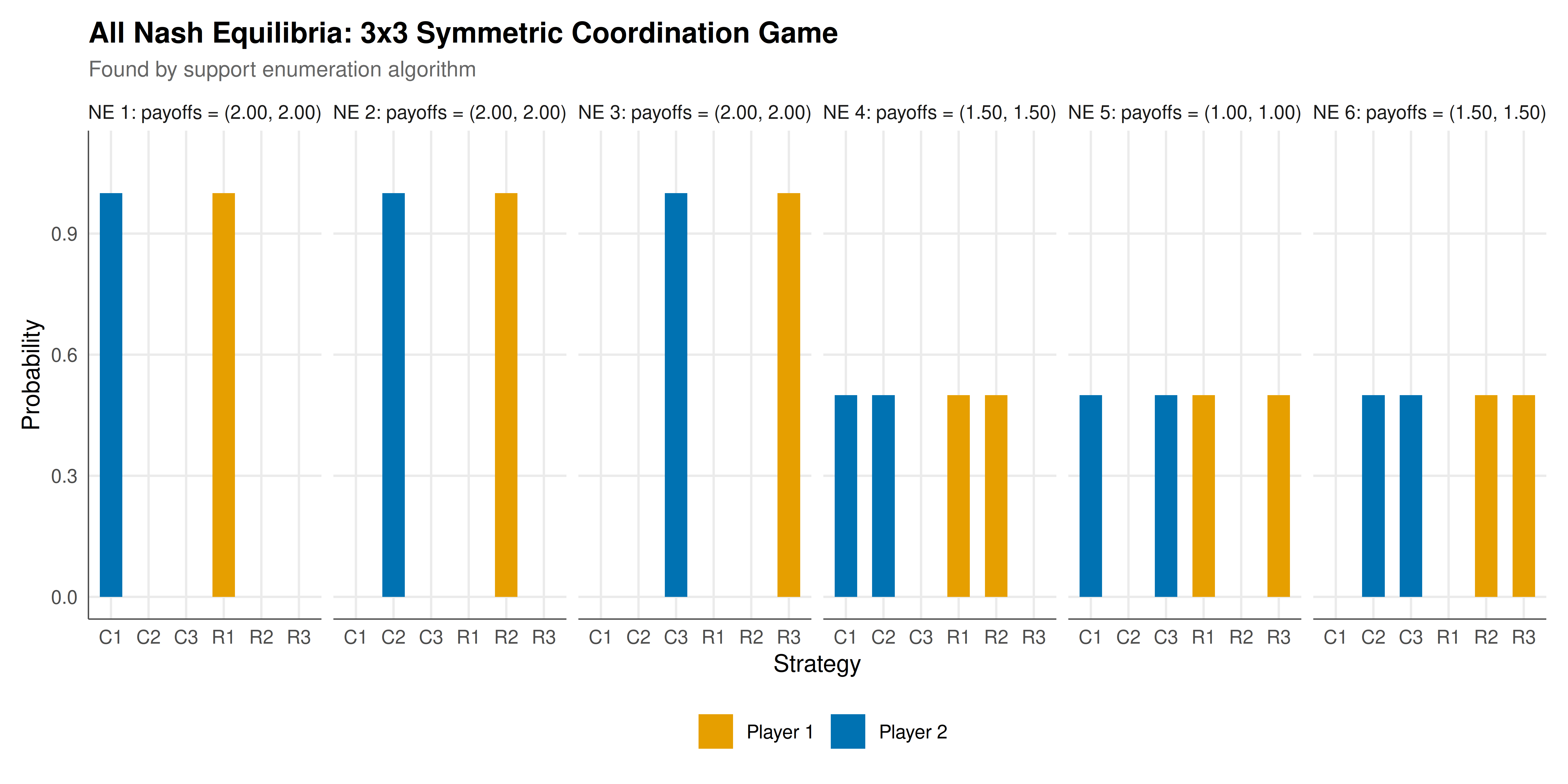
We visualise the support structure and probability weights of all Nash equilibria found for the 3x3 game, using a heatmap-style display that shows which strategies are in the support and with what probability.
```{r}
#| label: fig-support-enum-static
#| fig-cap: "Figure 1. Nash equilibria of the 3x3 symmetric coordination game found by support enumeration. Each panel shows the probability weights for one equilibrium. Pure equilibria concentrate all weight on a single strategy; the mixed equilibrium distributes weight across multiple strategies."
#| dev: [png, pdf]
#| fig-width: 10
#| fig-height: 5
#| dpi: 300
# Build data frame for all equilibria of Game 2
eq_plot_data <- data.frame()
for (i in seq_along(eq2)) {
  for (s in 1:3) {
    eq_plot_data <- rbind(eq_plot_data, data.frame(
      equilibrium = paste("NE", i),
      player = "Player 1",
      strategy = paste0("R", s),
      probability = eq2[[i]]$x[s]
    ))
    eq_plot_data <- rbind(eq_plot_data, data.frame(
      equilibrium = paste("NE", i),
      player = "Player 2",
      strategy = paste0("C", s),
      probability = eq2[[i]]$y[s]
    ))
  }
}

# Add payoff info to facet labels
eq_labels <- sapply(seq_along(eq2), function(i) {
  sprintf("NE %d: payoffs = (%.2f, %.2f)", i,
          eq2[[i]]$payoff_1, eq2[[i]]$payoff_2)
})
names(eq_labels) <- paste("NE", seq_along(eq2))
eq_plot_data$eq_label <- eq_labels[eq_plot_data$equilibrium]

p_support <- ggplot(eq_plot_data,
                    aes(x = strategy, y = probability, fill = player)) +
  geom_col(position = position_dodge(width = 0.7), width = 0.6) +
  facet_wrap(~eq_label, nrow = 1) +
  scale_fill_manual(values = okabe_ito[c(1, 5)], name = "") +
  labs(
    title = "All Nash Equilibria: 3x3 Symmetric Coordination Game",
    subtitle = "Found by support enumeration algorithm",
    x = "Strategy", y = "Probability"
  ) +
  theme_publication(base_size = 11) +
  coord_cartesian(ylim = c(0, 1.1))

p_support
```
## Interactive figure
The interactive figure shows the equilibria for the 4x4 game, allowing readers to explore the probability weights and support structure of each equilibrium by hovering.
```{r}
#| label: fig-support-enum-interactive
# Build data for Game 3 (4x4)
eq3_plot <- data.frame()
for (i in seq_along(eq3)) {
  for (s in 1:4) {
    eq3_plot <- rbind(eq3_plot, data.frame(
      equilibrium = paste("NE", i),
      player = "Player 1",
      strategy = paste0("R", s),
      probability = eq3[[i]]$x[s]
    ))
    eq3_plot <- rbind(eq3_plot, data.frame(
      equilibrium = paste("NE", i),
      player = "Player 2",
      strategy = paste0("C", s),
      probability = eq3[[i]]$y[s]
    ))
  }
}

eq3_plot <- eq3_plot %>%
  mutate(in_support = ifelse(probability > 1e-8, "Yes", "No"),
         label = sprintf("NE: %s\n%s: %s\nProbability: %.4f\nIn support: %s",
                         equilibrium, player, strategy,
                         probability, in_support))

p_int <- ggplot(eq3_plot,
                aes(x = strategy, y = probability, fill = player,
                    text = label)) +
  geom_col(position = position_dodge(width = 0.7), width = 0.6) +
  facet_wrap(~equilibrium, nrow = 1) +
  scale_fill_manual(values = okabe_ito[c(1, 5)], name = "") +
  labs(
    title = "Nash Equilibria of 4x4 Game (Interactive)",
    x = "Strategy", y = "Probability"
  ) +
  theme_publication(base_size = 10)

ggplotly(p_int, tooltip = "text") %>%
  config(displaylogo = FALSE)
```
## Interpretation
The support enumeration algorithm successfully finds all Nash equilibria in each of our test games, demonstrating both its correctness and the variety of equilibrium structures that can arise in bimatrix games.
For the Battle of the Sexes (Game 1), the algorithm finds the expected three equilibria: two pure strategy equilibria where both players coordinate on the same option (one preferring Opera, one preferring Football) and one mixed equilibrium where each player randomises. The mixed equilibrium has lower expected payoffs for both players than either pure equilibrium, illustrating the coordination problem: if neither player knows which pure equilibrium to play, the resulting randomisation leads to a positive probability of miscoordination.
The 3x3 symmetric coordination game (Game 2) reveals a richer structure. The pure equilibria place all probability on matching strategies, while the mixed equilibria (if any) distribute weight across strategies in the support. The indifference conditions that define each mixed equilibrium create a system of linear equations whose solution determines the exact mixing probabilities. The fact that different support pairs lead to different equilibria shows that the support structure is a fundamental property of each equilibrium, not just an incidental feature.
The 4x4 random game (Game 3) demonstrates the algorithm's scalability. With 225 support pairs to enumerate, the algorithm still runs in a fraction of a second. However, the exponential growth in support pairs ($2^m \cdot 2^n$ minus the empty sets) means that games much larger than $6 \times 6$ or $7 \times 7$ become computationally challenging. This is where the Lemke-Howson algorithm offers a practical advantage: it can find one Nash equilibrium efficiently even for larger games, at the cost of not guaranteeing to find all of them.
The trade-off between completeness and efficiency is fundamental. Support enumeration is the method of choice when you need all equilibria (for example, to select among them using refinement criteria or to verify uniqueness). The Lemke-Howson algorithm (and its modern variants) is preferred when one equilibrium suffices and the game is too large for full enumeration. For very large games, heuristic methods like fictitious play or regret-based learning may be the only practical option, though they do not provide exact equilibria.
## Extensions & related tutorials
The support enumeration approach extends naturally to more refined equilibrium concepts. By adding additional constraints to the enumeration (e.g., requiring trembling-hand perfection or sequential rationality), one can filter for specific refinements. For games with special structure (zero-sum, potential games), specialised algorithms are more efficient. The vertex enumeration approach to computing correlated equilibria provides a different perspective on the relationship between supports and equilibria.
- [LP duality and zero-sum game solutions](../../linear-algebra-matrix/lp-duality-zero-sum/)
- [Fictitious play and convergence](../../ml-and-gt/fictitious-play-convergence/)
- [Value of information in strategic games](../../information-theory/value-of-information-games/)
- [Congestion games and potential functions](../../network-games/congestion-games-potential/)
- [Diffusion and cascades on networks](../../network-science/diffusion-cascades-networks/)
## References
::: {#refs}
:::