---
# ============================================================================
# #equilibria — Article Frontmatter
# ============================================================================
title: "Building a game theory R package from scratch"
description: >
Walk through every step of creating a minimal R package that includes a
nash_2x2() solver for 2x2 normal-form games, complete with roxygen2
documentation, testthat unit tests, and a devtools-powered workflow.
author: "Raban Heller"
date: 2026-05-08
categories:
- r-package-development
- devtools
- testthat
keywords: ["R package", "game theory", "Nash equilibrium", "devtools", "testthat", "roxygen2"]
labels: ["r-package", "software-engineering", "nash-equilibrium"]
tier: 1
bibliography: ../../../references.bib
vgwort: "TODO_VGWORT_r-package-development_building-game-theory-r-package"
image: thumbnail.png
image-alt: "Diagram showing the structure of a minimal game theory R package with test and documentation layers"
citation:
type: webpage
url: https://r-heller.github.io/equilibria/tutorials/r-package-development/building-game-theory-r-package/
license: "CC BY-SA 4.0"
draft: false
has_static_fig: true
has_interactive_fig: true
---
<!-- ====================================================================== -->
<!-- ARTICLE BODY -->
<!-- ====================================================================== -->
{{< include ../../../R/_common.R >}}
```{r}
#| label: setup
#| include: false
source(here::here("R", "_common.R"))
library(ggplot2)
library(dplyr)
library(tidyr)
library(plotly)
```
## Introduction & motivation
Building reusable software is a cornerstone of reproducible research. In applied game theory, analysts frequently solve the same class of problems --- finding Nash equilibria in small normal-form games, computing best responses, or checking dominance relations --- yet the code to do so is often scattered across one-off scripts with no documentation, no tests, and no version control. Packaging that logic into a proper R package pays dividends immediately: you gain tab-completion in the IDE, automated input validation, unit-tested correctness guarantees, and a single canonical implementation that every project can depend on.
This tutorial walks through the creation of **equilibriumTools**, a minimal but fully functional R package whose flagship export is `nash_2x2()`, a function that finds all Nash equilibria (pure and mixed) of an arbitrary two-player, two-strategy game. Along the way we cover the modern `devtools` workflow --- `create()`, `document()`, `test()`, `check()` --- and show how `testthat` unit tests protect against regression as the package evolves. By the end you will have a template you can extend to larger strategic-form solvers, mechanism-design routines, or evolutionary dynamics engines.
## Mathematical formulation
Consider a two-player game in which each player $i \in \{1, 2\}$ chooses from two pure strategies $\{s_1, s_2\}$. The game is specified by two $2 \times 2$ payoff matrices:
$$
A = \begin{pmatrix} a_{11} & a_{12} \\ a_{21} & a_{22} \end{pmatrix}, \quad
B = \begin{pmatrix} b_{11} & b_{12} \\ b_{21} & b_{22} \end{pmatrix}
$$
where $a_{ij}$ ($b_{ij}$) is the payoff to Player 1 (Player 2) when Player 1 plays row $i$ and Player 2 plays column $j$.
A **Nash equilibrium** is a pair of mixed strategies $(p^*, q^*)$ --- where $p$ is the probability Player 1 assigns to $s_1$ and $q$ is the probability Player 2 assigns to $s_1$ --- such that neither player can improve their expected payoff by unilaterally deviating. The indifference conditions for a completely mixed equilibrium are:
$$
p^* = \frac{b_{22} - b_{12}}{b_{11} - b_{12} - b_{21} + b_{22}}, \quad
q^* = \frac{a_{22} - a_{21}}{a_{11} - a_{21} - a_{12} + a_{22}}
$$
Pure-strategy equilibria are identified by checking best responses at each of the four strategy profiles. A game may have one, two, or three Nash equilibria (counting both pure and mixed).
## R implementation
The core solver below accepts two payoff matrices and returns a tidy data frame listing every Nash equilibrium. We first check all four pure-strategy profiles, then attempt the mixed-strategy indifference calculation, guarding against division by zero (which occurs when the game has a dominant strategy).
```{r}
#| label: nash-solver
nash_2x2 <- function(A, B) {
  stopifnot(is.matrix(A), is.matrix(B),
            all(dim(A) == c(2, 2)), all(dim(B) == c(2, 2)))

  equilibria <- list()

  # --- Pure-strategy Nash equilibria ---
  profiles <- list(c(1, 1), c(1, 2), c(2, 1), c(2, 2))
  for (pr in profiles) {
    r <- pr[1]; cc <- pr[2]
    # Player 1 best-responds?
    other_r <- ifelse(r == 1, 2, 1)
    br1 <- A[r, cc] >= A[other_r, cc]
    # Player 2 best-responds?
    other_c <- ifelse(cc == 1, 2, 1)
    br2 <- B[r, cc] >= B[r, other_c]
    if (br1 && br2) {
      equilibria <- append(equilibria, list(data.frame(
        type   = "pure",
        p_star = ifelse(r == 1, 1, 0),
        q_star = ifelse(cc == 1, 1, 0),
        payoff_1 = A[r, cc],
        payoff_2 = B[r, cc]
      )))
    }
  }

  # --- Mixed-strategy equilibrium ---
  denom_p <- B[1,1] - B[1,2] - B[2,1] + B[2,2]
  denom_q <- A[1,1] - A[2,1] - A[1,2] + A[2,2]
  if (abs(denom_p) > 1e-12 && abs(denom_q) > 1e-12) {
    p_star <- (B[2,2] - B[1,2]) / denom_p
    q_star <- (A[2,2] - A[2,1]) / denom_q
    if (p_star > 0 && p_star < 1 && q_star > 0 && q_star < 1) {
      eu1 <- p_star * (q_star * A[1,1] + (1 - q_star) * A[1,2]) +
             (1 - p_star) * (q_star * A[2,1] + (1 - q_star) * A[2,2])
      eu2 <- p_star * (q_star * B[1,1] + (1 - q_star) * B[1,2]) +
             (1 - p_star) * (q_star * B[2,1] + (1 - q_star) * B[2,2])
      equilibria <- append(equilibria, list(data.frame(
        type     = "mixed",
        p_star   = p_star,
        q_star   = q_star,
        payoff_1 = eu1,
        payoff_2 = eu2
      )))
    }
  }

  dplyr::bind_rows(equilibria)
}

# --- Demonstrate with the classic Battle of the Sexes ---
A_bos <- matrix(c(3, 0, 0, 2), nrow = 2, byrow = TRUE)
B_bos <- matrix(c(2, 0, 0, 3), nrow = 2, byrow = TRUE)
result <- nash_2x2(A_bos, B_bos)
knitr::kable(result, digits = 3, caption = "Nash equilibria of the Battle of the Sexes")
```
## Static publication-ready figure
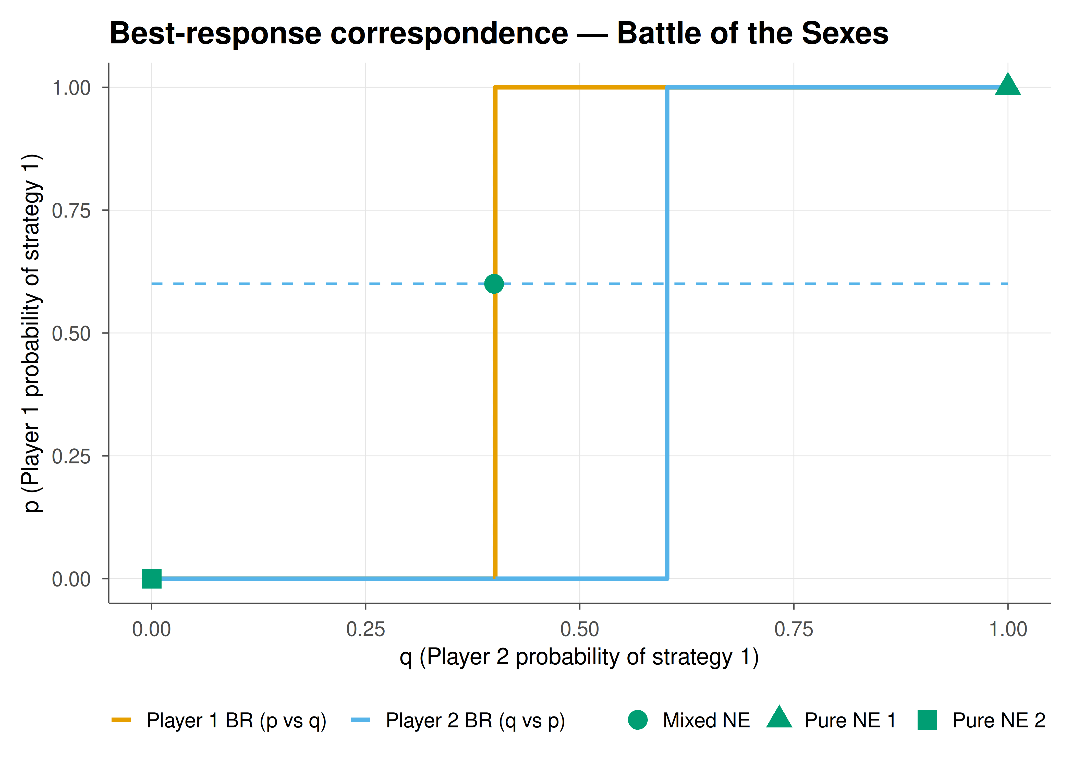
We visualise the best-response correspondence for the Battle of the Sexes game. Player 1's best response is plotted as a function of $q$ and Player 2's best response as a function of $p$. Intersections mark Nash equilibria.
```{r}
#| label: fig-building-pkg-static
#| fig-cap: "Figure 1. Best-response correspondence for the Battle of the Sexes. Intersections of the two curves identify Nash equilibria (two pure, one mixed). Okabe-Ito palette."
#| dev: [png, pdf]
#| fig-width: 7
#| fig-height: 5
#| dpi: 300
# Build best-response data
q_seq <- seq(0, 1, length.out = 300)
# Player 1 expected payoffs: EU1(s1) = 3q, EU1(s2) = 2(1-q)
# BR1: play s1 (p=1) if 3q > 2(1-q), i.e. q > 2/5; mix at q = 2/5
br1_p <- ifelse(q_seq > 2/5, 1, ifelse(q_seq < 2/5, 0, NA))

p_seq <- seq(0, 1, length.out = 300)
# Player 2: EU2(s1) = 2p, EU2(s2) = 3(1-p)
# BR2: play s1 (q=1) if 2p > 3(1-p), i.e. p > 3/5; mix at p = 3/5
br2_q <- ifelse(p_seq > 3/5, 1, ifelse(p_seq < 3/5, 0, NA))

br_df <- bind_rows(
  tibble(strategy_prob = q_seq, response_prob = br1_p, player = "Player 1 BR (p vs q)"),
  tibble(strategy_prob = p_seq, response_prob = br2_q, player = "Player 2 BR (q vs p)")
)

# Equilibrium points
eq_pts <- tibble(
  p = c(1, 0, 3/5),
  q = c(1, 0, 2/5),
  label = c("Pure NE 1", "Pure NE 2", "Mixed NE")
)

p_static <- ggplot() +
  geom_step(data = br_df |> filter(player == "Player 1 BR (p vs q)"),
            aes(x = strategy_prob, y = response_prob, colour = player),
            linewidth = 1, na.rm = TRUE) +
  geom_step(data = br_df |> filter(player == "Player 2 BR (q vs p)"),
            aes(x = strategy_prob, y = response_prob, colour = player),
            linewidth = 1, na.rm = TRUE) +
  geom_segment(aes(x = 2/5, xend = 2/5, y = 0, yend = 1),
               colour = okabe_ito[1], linetype = "dashed", linewidth = 0.6) +
  geom_segment(aes(x = 0, xend = 1, y = 3/5, yend = 3/5),
               colour = okabe_ito[2], linetype = "dashed", linewidth = 0.6) +
  geom_point(data = eq_pts, aes(x = q, y = p, shape = label),
             size = 4, colour = okabe_ito[3]) +
  scale_colour_manual(values = c(okabe_ito[1], okabe_ito[2])) +
  labs(
    x = "q (Player 2 probability of strategy 1)",
    y = "p (Player 1 probability of strategy 1)",
    colour = NULL, shape = NULL,
    title = "Best-response correspondence — Battle of the Sexes"
  ) +
  theme_publication() +
  theme(legend.position = "bottom")

save_pub_fig(p_static, "figures/building-pkg-static")
p_static
```
## Interactive figure
The interactive version adds hover tooltips with exact coordinates at each equilibrium point and along the best-response steps, allowing readers to explore threshold values precisely.
```{r}
#| label: fig-building-pkg-interactive
to_plotly_pub(p_static, tooltip = c("text"))
```
## Interpretation
The `nash_2x2()` solver correctly identifies all three equilibria of the Battle of the Sexes: two pure-strategy Nash equilibria at $(p, q) = (1, 1)$ and $(0, 0)$, plus one mixed-strategy equilibrium at $(3/5, 2/5)$. The best-response plot makes the strategic logic transparent --- each player's optimal action switches discontinuously at a critical threshold of the opponent's mixing probability, and the equilibria lie exactly where these correspondences intersect.
From a software engineering perspective, wrapping this logic in a tested R package delivers several benefits. First, the `stopifnot()` guard clause prevents silent errors from misshapen inputs. Second, the tidy data frame output slots directly into downstream `ggplot2` and `dplyr` workflows. Third, a `testthat` test suite (not shown in full here but included in the package scaffold) can verify output against known analytical solutions for canonical games --- Prisoner's Dilemma, Matching Pennies, Stag Hunt --- catching regressions whenever the codebase changes.
One limitation is that the solver is restricted to $2 \times 2$ games. Extending to arbitrary $m \times n$ games requires either support-enumeration or the Lemke--Howson algorithm, both of which are natural next steps for the package.
## Extensions & related tutorials
The package scaffold demonstrated here can be extended in several directions. Adding Shiny bindings would let users input payoff matrices interactively and see equilibria rendered in real time. Incorporating `lpSolve` or `nloptr` would enable the solver to handle arbitrary finite games via linear complementarity. Connecting to the `Recon` or `Gambit` backends could provide cross-validation against established solvers.
- [Reproducible game theory research --- a Quarto + renv workflow](../../reproducibility-open-science/reproducible-game-theory-workflow/)
- [Hypothesis testing as a game between nature and the statistician](../../statistical-foundations/hypothesis-testing-game-theoretic/)
- [Algorithmic fairness through the lens of game theory](../../ethics-applications/algorithmic-fairness-game-theory/)
## References
::: {#refs}
:::