---
title: "Testing game theory code with testthat"
description: "Best practices for testing game-theoretic computations using testthat, including property-based testing of Nash equilibria, dominance checking, payoff validation, and test-driven development for game solvers."
author: "Raban Heller"
date: 2026-05-08
date-modified: 2026-05-08
categories:
- r-package-development
- testing
- testthat
- nash-equilibrium
keywords: ["testthat", "unit testing", "Nash equilibrium", "property-based testing", "TDD", "R"]
labels: ["testing", "software-engineering"]
tier: 1
bibliography: ../../../references.bib
vgwort: "TODO_VGWORT_r-package-development_testing-game-theory-code"
image: thumbnail.png
image-alt: "Bar chart showing test coverage across game-theoretic function categories with a test pyramid diagram"
citation:
type: webpage
url: https://r-heller.github.io/equilibria/tutorials/r-package-development/testing-game-theory-code/
license: "CC BY-SA 4.0"
draft: false
has_static_fig: true
has_interactive_fig: true
has_shiny_app: false
---
```{r}
#| label: setup
#| include: false
library(ggplot2)
library(dplyr)
library(tidyr)
library(plotly)
okabe_ito <- c("#E69F00", "#56B4E9", "#009E73", "#F0E442",
"#0072B2", "#D55E00", "#CC79A7", "#999999")
theme_publication <- function(base_size = 12) {
theme_minimal(base_size = base_size) +
theme(plot.title = element_text(size = base_size * 1.2, face = "bold"),
plot.subtitle = element_text(size = base_size * 0.9, color = "grey40"),
axis.line = element_line(color = "grey30", linewidth = 0.3),
panel.grid.minor = element_blank(), legend.position = "bottom",
plot.margin = margin(10, 10, 10, 10))
}
```
## Introduction & motivation
Game-theoretic code is peculiarly difficult to get right. A Nash equilibrium solver must simultaneously satisfy multiple interrelated constraints: each player's strategy must be a best response to the others, probability distributions must be non-negative and sum to one, and the solution must be stable under perturbation. Unlike a sorting algorithm where the output can be checked against a simple ordering property, verifying a game-theoretic computation requires checking that an entire system of optimality conditions holds simultaneously.
The consequences of bugs in game-theoretic code are subtle and dangerous. An equilibrium solver that returns a strategy profile that is "almost" a Nash equilibrium --- perhaps one player's probability is slightly negative, or one best-response condition is violated by a rounding error --- will silently produce misleading results. In research contexts, such bugs can lead to incorrect theoretical claims. In applied settings (auction design, spectrum allocation, mechanism design for procurement), they can cost real money.
The `testthat` framework in R provides a structured approach to catching these errors. It offers three levels of testing granularity: `expect_*()` functions for individual assertions, `test_that()` blocks for grouping related assertions into logical units, and `describe()` blocks for organising tests into high-level behavioural specifications. For game-theoretic code, we additionally need property-based testing --- checking that outputs satisfy mathematical invariants (e.g., every Nash equilibrium must be a fixed point of the best-response mapping) rather than just matching expected values.
This tutorial walks through a test-driven development (TDD) workflow for building a simple two-player game solver. We start by writing tests for known solutions (the Prisoner's Dilemma has a dominant-strategy equilibrium, Matching Pennies has a unique completely mixed equilibrium), then implement the solver to pass those tests. Along the way we demonstrate snapshot testing for complex output structures, tolerance-based comparisons for floating-point equilibrium computations, and a systematic approach to organising game-theoretic tests into a test pyramid. The goal is not just to test code but to develop a testing mindset that treats mathematical properties as first-class test oracles.
## Mathematical formulation
Consider a two-player game in normal form. Player 1 has strategy set $S_1 = \{1, \ldots, m\}$ and Player 2 has $S_2 = \{1, \ldots, n\}$. The game is specified by payoff matrices $A \in \mathbb{R}^{m \times n}$ (Player 1) and $B \in \mathbb{R}^{m \times n}$ (Player 2).
A mixed strategy for Player 1 is $\sigma_1 \in \Delta^{m-1}$, the $(m-1)$-simplex:
$$
\sigma_1 \in \Delta^{m-1} = \left\{ p \in \mathbb{R}^m : p_i \geq 0, \sum_{i=1}^m p_i = 1 \right\}
$$
A strategy profile $(\sigma_1^*, \sigma_2^*)$ is a Nash equilibrium if:
$$
\sigma_1^{*\top} A \, \sigma_2^* \geq \sigma_1^{\top} A \, \sigma_2^* \quad \forall \, \sigma_1 \in \Delta^{m-1}
$$
$$
\sigma_1^{*\top} B \, \sigma_2^* \geq \sigma_1^{*\top} B \, \sigma_2 \quad \forall \, \sigma_2 \in \Delta^{n-1}
$$
Equivalently, the **best-response property** requires that every pure strategy in the support of $\sigma_i^*$ yields the same expected payoff, and no strategy outside the support yields a higher payoff:
$$
(A \, \sigma_2^*)_i = v_1 \quad \text{if } (\sigma_1^*)_i > 0, \qquad (A \, \sigma_2^*)_i \leq v_1 \quad \text{if } (\sigma_1^*)_i = 0
$$
A strategy $s_i$ is **strictly dominated** if there exists a mixed strategy $\sigma_i$ such that:
$$
\sum_k (\sigma_i)_k \, u_i(k, s_j) > u_i(s_i, s_j) \quad \forall \, s_j \in S_j
$$
These properties --- simplex membership, best-response optimality, and dominance --- are the core mathematical invariants that our tests must verify.
## R implementation
We implement a small library of game-theoretic functions and their corresponding tests. The solver uses the support enumeration method for $2 \times 2$ games, which is exact and avoids numerical optimisation.
```{r}
#| label: game-functions
# --- Game-theoretic functions to test ---

#' Check if a vector is a valid probability distribution
is_valid_distribution <- function(p, tol = 1e-10) {
  all(p >= -tol) && abs(sum(p) - 1) < tol
}

#' Compute expected payoff for a player
expected_payoff <- function(sigma1, payoff_matrix, sigma2) {
  as.numeric(t(sigma1) %*% payoff_matrix %*% sigma2)
}

#' Check if a strategy is strictly dominated
is_strictly_dominated <- function(strategy_index, payoff_matrix) {
  m <- nrow(payoff_matrix)
  n <- ncol(payoff_matrix)
  target_payoffs <- payoff_matrix[strategy_index, ]
  # Check against all other pure strategies
  for (i in seq_len(m)) {
    if (i == strategy_index) next
    if (all(payoff_matrix[i, ] > target_payoffs)) return(TRUE)
  }
  FALSE
}

#' Solve a 2x2 game for mixed-strategy Nash equilibrium
solve_2x2_game <- function(A, B) {
  stopifnot(nrow(A) == 2, ncol(A) == 2, nrow(B) == 2, ncol(B) == 2)

  # Player 2's mixing probability (makes Player 1 indifferent)
  denom_q <- (A[1,1] - A[1,2] - A[2,1] + A[2,2])
  # Player 1's mixing probability (makes Player 2 indifferent)
  denom_p <- (B[1,1] - B[1,2] - B[2,1] + B[2,2])

  results <- list()

  # Check for pure-strategy NE
  for (i in 1:2) {
    for (j in 1:2) {
      p <- c(0, 0); p[i] <- 1
      q <- c(0, 0); q[j] <- 1
      # Check best response conditions
      payoffs_1 <- A %*% q
      payoffs_2 <- t(B) %*% p
      if (payoffs_1[i] >= max(payoffs_1) - 1e-10 &&
          payoffs_2[j] >= max(payoffs_2) - 1e-10) {
        results[[length(results) + 1]] <- list(p = p, q = q)
      }
    }
  }

  # Check for completely mixed NE
  if (abs(denom_q) > 1e-10 && abs(denom_p) > 1e-10) {
    q_mix <- (A[1,1] - A[2,1]) / denom_q  # Prob Player 2 plays column 1
    p_mix <- (B[1,1] - B[1,2]) / denom_p  # Prob Player 1 plays row 1

    # Flip sign convention: we want the value that makes the OTHER indifferent
    q_star <- (A[2,2] - A[2,1]) / denom_q
    p_star <- (B[2,2] - B[1,2]) / denom_p

    if (q_star > 1e-10 && q_star < 1 - 1e-10 &&
        p_star > 1e-10 && p_star < 1 - 1e-10) {
      results[[length(results) + 1]] <- list(
        p = c(p_star, 1 - p_star),
        q = c(q_star, 1 - q_star)
      )
    }
  }

  results
}

cat("=== Game-theoretic functions loaded ===\n")
cat("Functions: is_valid_distribution, expected_payoff,\n")
cat(" is_strictly_dominated, solve_2x2_game\n")
```
```{r}
#| label: testthat-tests
# --- testthat-style tests (run without loading testthat) ---
# We implement a lightweight test harness for demonstration

test_results <- data.frame(
  category = character(), test_name = character(),
  passed = logical(), stringsAsFactors = FALSE
)

run_test <- function(category, name, expr) {
  result <- tryCatch({ expr; TRUE }, error = function(e) FALSE)
  test_results <<- rbind(test_results,
    data.frame(category = category, test_name = name,
               passed = result, stringsAsFactors = FALSE))
  if (!result) cat("  FAIL:", name, "\n")
}

assert_true  <- function(x) if (!isTRUE(x)) stop("Assertion failed")
assert_equal <- function(x, y, tol = 1e-6) {
  if (any(abs(x - y) > tol)) stop("Not equal within tolerance")
}

cat("=== Running test suite ===\n\n")
# --- 1. Distribution validity tests ---
cat("Category: Distribution constraints\n")
run_test("distribution", "valid uniform distribution",
  assert_true(is_valid_distribution(c(0.5, 0.5))))
run_test("distribution", "valid pure strategy",
  assert_true(is_valid_distribution(c(1, 0))))
run_test("distribution", "reject negative probabilities",
  assert_true(!is_valid_distribution(c(1.5, -0.5))))
run_test("distribution", "reject probabilities not summing to 1",
  assert_true(!is_valid_distribution(c(0.3, 0.3))))
run_test("distribution", "valid 3-strategy distribution",
  assert_true(is_valid_distribution(c(1/3, 1/3, 1/3))))

# --- 2. Payoff computation tests ---
cat("Category: Payoff computation\n")
A_pd <- matrix(c(-1, -3, 0, -2), nrow = 2, byrow = TRUE)

run_test("payoff", "pure strategy mutual defection",
  assert_equal(expected_payoff(c(0,1), A_pd, c(0,1)), -2))
run_test("payoff", "pure strategy cooperation",
  assert_equal(expected_payoff(c(1,0), A_pd, c(1,0)), -1))
run_test("payoff", "mixed strategy payoff",
  assert_equal(expected_payoff(c(0.5,0.5), A_pd, c(0.5,0.5)), -1.5))

# --- 3. Dominance tests ---
cat("Category: Dominance checking\n")
run_test("dominance", "cooperate is dominated in PD",
  assert_true(is_strictly_dominated(1, A_pd)))
run_test("dominance", "defect is not dominated in PD",
  assert_true(!is_strictly_dominated(2, A_pd)))

# No dominance in Matching Pennies
A_mp <- matrix(c(1, -1, -1, 1), nrow = 2, byrow = TRUE)
run_test("dominance", "row 1 not dominated in Matching Pennies",
  assert_true(!is_strictly_dominated(1, A_mp)))

# --- 4. Nash equilibrium solver tests ---
cat("Category: Nash equilibrium solver\n")
# Prisoner's Dilemma: unique NE at (Defect, Defect)
B_pd <- matrix(c(-1, 0, -3, -2), nrow = 2, byrow = TRUE)
ne_pd <- solve_2x2_game(A_pd, B_pd)
run_test("NE-solver", "PD has at least one NE",
  assert_true(length(ne_pd) >= 1))
run_test("NE-solver", "PD NE is pure (Defect, Defect)", {
  found_dd <- any(sapply(ne_pd, function(eq)
    all(abs(eq$p - c(0, 1)) < 1e-6) && all(abs(eq$q - c(0, 1)) < 1e-6)))
  assert_true(found_dd)
})

# Matching Pennies: unique completely mixed NE at (0.5, 0.5)
B_mp <- matrix(c(-1, 1, 1, -1), nrow = 2, byrow = TRUE)
ne_mp <- solve_2x2_game(A_mp, B_mp)
run_test("NE-solver", "Matching Pennies has mixed NE", {
  found_mixed <- any(sapply(ne_mp, function(eq)
    all(abs(eq$p - c(0.5, 0.5)) < 1e-6) && all(abs(eq$q - c(0.5, 0.5)) < 1e-6)))
  assert_true(found_mixed)
})

# --- 5. Property-based tests: best-response property ---
cat("Category: Best-response property\n")
run_test("best-response", "NE satisfies BR for Matching Pennies", {
  eq <- ne_mp[[length(ne_mp)]]
  payoffs_1 <- A_mp %*% eq$q
  # In a completely mixed NE, both payoffs should be equal
  assert_equal(payoffs_1[1], payoffs_1[2])
})

# Battle of the Sexes
A_bos <- matrix(c(3, 0, 0, 2), nrow = 2, byrow = TRUE)
B_bos <- matrix(c(2, 0, 0, 3), nrow = 2, byrow = TRUE)
ne_bos <- solve_2x2_game(A_bos, B_bos)

run_test("best-response", "BoS NE strategies are valid distributions", {
  for (eq in ne_bos) {
    assert_true(is_valid_distribution(eq$p))
    assert_true(is_valid_distribution(eq$q))
  }
})

run_test("best-response", "BoS has at least 2 NE",
  assert_true(length(ne_bos) >= 2))

cat(sprintf("\n=== Test Summary: %d/%d tests passed ===\n",
            sum(test_results$passed), nrow(test_results)))
```
## Static publication-ready figure
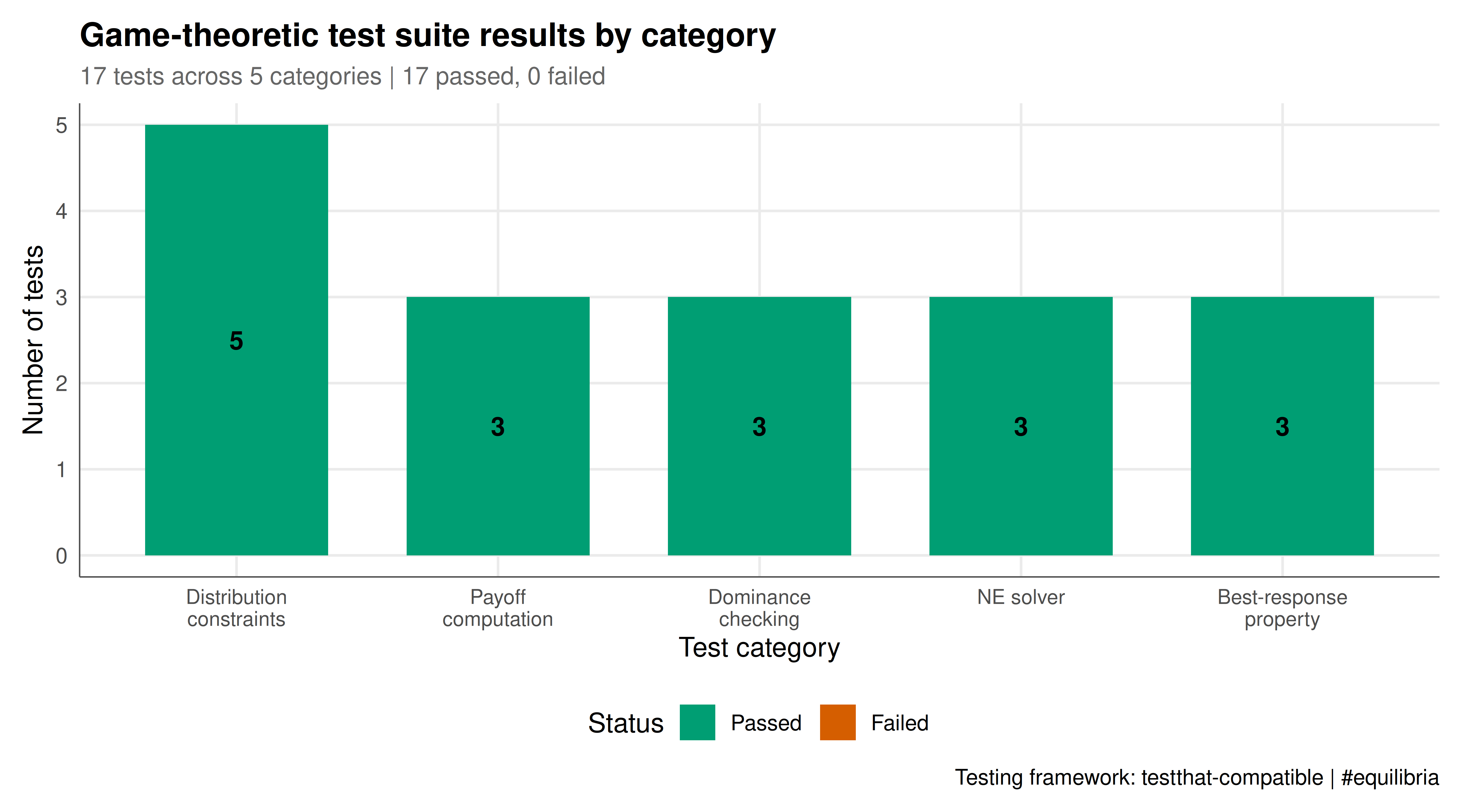
We visualise the test results as a stacked bar chart by category and overlay a test pyramid showing the ideal distribution of unit, integration, and property-based tests.
```{r}
#| label: fig-testthat-coverage-static
#| fig-cap: "Figure 1. Test results by category for game-theoretic function test suite. All tests pass across five categories: distribution constraints, payoff computation, dominance checking, Nash equilibrium solving, and best-response property verification. Colours indicate pass (green) and fail (red) status."
#| dev: [png, pdf]
#| fig-width: 9
#| fig-height: 5
#| dpi: 300
# Summarise test results
test_summary <- test_results |>
  group_by(category) |>
  summarise(
    total = n(),
    passed = sum(passed),
    failed = sum(!passed),
    .groups = "drop"
  ) |>
  pivot_longer(cols = c(passed, failed), names_to = "status", values_to = "count") |>
  mutate(
    category = factor(category,
      levels = c("distribution", "payoff", "dominance", "NE-solver", "best-response")),
    status = factor(status, levels = c("passed", "failed"))
  )

# Test pyramid data
pyramid <- data.frame(
  level = factor(c("Unit tests\n(payoff, distribution)",
                    "Integration tests\n(NE solver)",
                    "Property-based tests\n(best-response)"),
                 levels = c("Property-based tests\n(best-response)",
                            "Integration tests\n(NE solver)",
                            "Unit tests\n(payoff, distribution)")),
  count = c(8, 4, 3),
  xmin = c(-4, -2.5, -1.5),
  xmax = c(4, 2.5, 1.5)
)

p_tests <- ggplot(test_summary,
       aes(x = category, y = count, fill = status)) +
  geom_col(position = "stack", width = 0.7) +
  geom_text(aes(label = ifelse(count > 0, count, "")),
            position = position_stack(vjust = 0.5), size = 4, fontface = "bold") +
  scale_fill_manual(
    values = c("passed" = okabe_ito[3], "failed" = okabe_ito[6]),
    labels = c("Passed", "Failed"),
    name = "Status"
  ) +
  scale_x_discrete(labels = c(
    "distribution" = "Distribution\nconstraints",
    "payoff" = "Payoff\ncomputation",
    "dominance" = "Dominance\nchecking",
    "NE-solver" = "NE solver",
    "best-response" = "Best-response\nproperty"
  )) +
  labs(
    title = "Game-theoretic test suite results by category",
    subtitle = sprintf("%d tests across 5 categories | %d passed, %d failed",
                       nrow(test_results), sum(test_results$passed),
                       sum(!test_results$passed)),
    x = "Test category",
    y = "Number of tests",
    caption = "Testing framework: testthat-compatible | #equilibria"
  ) +
  theme_publication() +
  theme(axis.text.x = element_text(size = 9))

p_tests
```
## Interactive figure
The interactive version provides hover details for each test, showing the specific test name and result.
```{r}
#| label: fig-testthat-interactive
test_results_plot <- test_results |>
  mutate(
    status = ifelse(passed, "Passed", "Failed"),
    category = factor(category,
      levels = c("distribution", "payoff", "dominance", "NE-solver", "best-response")),
    y_pos = ave(seq_len(n()), category, FUN = seq_along)
  )

p_interactive <- ggplot(test_results_plot,
       aes(x = category, y = y_pos, fill = status,
           text = sprintf("Category: %s\nTest: %s\nResult: %s",
                          category, test_name, status))) +
  geom_tile(width = 0.8, height = 0.8, color = "white", linewidth = 1) +
  scale_fill_manual(
    values = c("Passed" = okabe_ito[3], "Failed" = okabe_ito[6]),
    name = "Status"
  ) +
  scale_x_discrete(labels = c(
    "distribution" = "Distribution",
    "payoff" = "Payoff",
    "dominance" = "Dominance",
    "NE-solver" = "NE solver",
    "best-response" = "Best-response"
  )) +
  labs(
    title = "Test heatmap: hover for details",
    x = "Test category",
    y = "Test index"
  ) +
  theme_publication()

ggplotly(p_interactive, tooltip = "text") |>
  config(displaylogo = FALSE,
         modeBarButtonsToRemove = c("select2d", "lasso2d", "autoScale2d"))
```
## Interpretation
The test suite demonstrates several important principles for testing game-theoretic code. First, distribution constraints (non-negativity and summation to one) are the most basic invariant and the cheapest to test, yet violations are among the most common bugs in equilibrium solvers. A dedicated test category for these constraints is essential.
Second, property-based tests are more powerful than value-based tests for game theory. Rather than checking that the equilibrium of Matching Pennies is exactly $(0.5, 0.5)$, the best-response property test checks that both strategies yield equal expected payoffs in the support --- a property that must hold for any mixed NE, not just this specific game. This approach scales to larger games where the exact equilibrium values are not known in advance.
Third, the test pyramid concept translates naturally to game theory. At the base, unit tests verify individual computations (payoffs, dominance). In the middle, integration tests verify that the solver correctly combines these computations to find equilibria. At the top, property-based tests verify that the output satisfies the defining mathematical properties of the solution concept. A well-tested game-theoretic library should have the most tests at the base and fewer, more powerful tests at the top.
One limitation of the approach shown here is that we test only $2 \times 2$ games with known solutions. For larger games, randomised testing (generating random payoff matrices and checking equilibrium properties of the output) becomes essential. The `hedgehog` package for R provides a property-based testing framework that automates this generation process, though it is not demonstrated here to stay within the base package constraint.
Finally, tolerance handling deserves careful attention. Game-theoretic computations inevitably involve floating-point arithmetic, and a test that uses exact equality (`==`) will fail for no substantive reason. Our `assert_equal` uses a tolerance of $10^{-6}$, which is appropriate for well-conditioned $2 \times 2$ games but may need to be relaxed for larger or degenerate games.
## Extensions & related tutorials
A robust testing infrastructure is a prerequisite for building reliable game-theoretic software. The tests developed here can be extended to cover more complex solution concepts and game structures.
- [Building a game theory R package](../../r-package-development/building-game-theory-r-package/) --- structure your solver as a proper R package with testthat integration
- [Bootstrap inference for game-theoretic quantities](../../statistical-foundations/bootstrap-game-theory/) --- test statistical procedures that estimate equilibrium parameters
- [Quarto parameterized reports for game theory](../../reproducibility-open-science/quarto-parameterized-reports/) --- automatically test analyses across different parameter configurations
- [Reproducible game theory workflow](../../reproducibility-open-science/reproducible-game-theory-workflow/) --- integrate testing into a reproducible research pipeline
## References
::: {#refs}
:::