---
title: "Quarto parameterized reports for game theory"
description: "Use Quarto's params feature to create reusable game theory analyses that render multiple game variants --- Prisoner's Dilemma, Battle of the Sexes, Chicken --- from a single parameterized template."
author: "Raban Heller"
date: 2026-05-08
date-modified: 2026-05-08
categories:
- reproducibility-open-science
- quarto
- parameterized-reports
- reproducibility
keywords: ["Quarto", "parameterized reports", "reproducibility", "2x2 games", "batch rendering", "R"]
labels: ["reproducibility", "workflow"]
tier: 1
bibliography: ../../../references.bib
vgwort: "TODO_VGWORT_reproducibility-open-science_quarto-parameterized-reports"
image: thumbnail.png
image-alt: "Grid of four game-theoretic equilibrium diagrams generated from different parameter sets using a single Quarto template"
citation:
type: webpage
url: https://r-heller.github.io/equilibria/tutorials/reproducibility-open-science/quarto-parameterized-reports/
license: "CC BY-SA 4.0"
draft: false
has_static_fig: true
has_interactive_fig: true
has_shiny_app: false
---
```{r}
#| label: setup
#| include: false
library(ggplot2)
library(dplyr)
library(tidyr)
library(plotly)
okabe_ito <- c("#E69F00", "#56B4E9", "#009E73", "#F0E442",
"#0072B2", "#D55E00", "#CC79A7", "#999999")
theme_publication <- function(base_size = 12) {
theme_minimal(base_size = base_size) +
theme(plot.title = element_text(size = base_size * 1.2, face = "bold"),
plot.subtitle = element_text(size = base_size * 0.9, color = "grey40"),
axis.line = element_line(color = "grey30", linewidth = 0.3),
panel.grid.minor = element_blank(), legend.position = "bottom",
plot.margin = margin(10, 10, 10, 10))
}
```
## Introduction & motivation
One of the recurring tasks in game theory pedagogy and research is analysing the same class of game under different payoff configurations. A $2 \times 2$ symmetric game, for instance, can encode the Prisoner's Dilemma, the Stag Hunt, the Battle of the Sexes, or Chicken, depending on the specific payoff values chosen. Each variant has a different equilibrium structure: some have a unique dominant-strategy equilibrium, others have multiple pure-strategy equilibria and a mixed equilibrium, and some have only a mixed equilibrium. Manually rewriting an analysis document for each variant is tedious, error-prone, and violates the DRY (Don't Repeat Yourself) principle.
Quarto's parameterized reports offer an elegant solution. By declaring a set of `params` in the YAML front matter, you create a single template document that can be rendered with different parameter values to produce different analyses. Each rendering is fully self-contained and reproducible: the same code, the same analysis structure, but different data. This is the game-theoretic equivalent of a parameterized statistical report --- instead of varying sample sizes or treatment effects, we vary payoff matrix entries and observe how equilibrium structure changes.
The reproducibility benefits are substantial. When a referee asks "what happens if you change the temptation payoff from 5 to 7?", you do not need to hunt through your code for hard-coded values. You simply re-render with the new parameter. When teaching, you can generate a complete set of canonical $2 \times 2$ games from a single template, ensuring visual and analytical consistency across all examples. And when conducting comparative statics --- systematically varying one parameter while holding others fixed --- batch rendering produces a complete family of analyses with a single command.
In this tutorial we build a parameterized analysis of $2 \times 2$ games. The template accepts four payoff entries as parameters, computes all Nash equilibria (pure and mixed), classifies the game type, and produces both static and interactive visualisations of the best-response correspondences. We then demonstrate batch rendering for four canonical games, showing how different parameter combinations produce fundamentally different equilibrium landscapes.
The approach extends naturally to larger games, repeated games with discount factors as parameters, or mechanism design problems where the designer's choice variables become report parameters. The key insight is that parameterization separates the analysis logic (which is validated once) from the specific numerical inputs (which can be varied freely), dramatically reducing the risk of copy-paste errors.
## Mathematical formulation
We consider a symmetric $2 \times 2$ game with payoff matrix for each player:
$$
\begin{pmatrix} R & S \\ T & P \end{pmatrix}
$$
where $R$ (Reward) is the mutual cooperation payoff, $T$ (Temptation) is the defection-against-cooperator payoff, $S$ (Sucker) is the cooperator-against-defector payoff, and $P$ (Punishment) is the mutual defection payoff.
Let Player 1 play row 1 (Cooperate) with probability $p$ and Player 2 play column 1 (Cooperate) with probability $q$. The expected payoffs are:
$$
U_1(p, q) = pq \cdot R + p(1-q) \cdot S + (1-p)q \cdot T + (1-p)(1-q) \cdot P
$$
Player 1's best-response function is:
$$
p^*(q) = \begin{cases}
1 & \text{if } q(R - T) + (1-q)(S - P) > 0 \\
[0,1] & \text{if } q(R - T) + (1-q)(S - P) = 0 \\
0 & \text{if } q(R - T) + (1-q)(S - P) < 0
\end{cases}
$$
The indifference condition for Player 1 yields:
$$
q^* = \frac{P - S}{(R - T) + (P - S)} = \frac{P - S}{R - T + P - S}
$$
By symmetry, Player 2's indifference probability is:
$$
p^* = \frac{P - S}{R - T + P - S}
$$
A mixed-strategy NE exists at $(p^*, q^*)$ whenever $0 < p^* < 1$ and $0 < q^* < 1$. The game classification depends on the ordering of $R, S, T, P$:
- **Prisoner's Dilemma**: $T > R > P > S$
- **Stag Hunt**: $R > T > P > S$
- **Chicken (Hawk-Dove)**: $T > R > S > P$
- **Harmony**: $R > T > S > P$
## R implementation
We implement the parameterized game analysis engine. In a real Quarto parameterized report, the values of `R_val`, `T_val`, `S_val`, `P_val` would come from `params$R`, `params$T`, `params$S`, `params$P` in the YAML header. Here we demonstrate the logic by defining a reusable analysis function and applying it to multiple game configurations.
```{r}
#| label: parameterized-analysis-engine
# --- Parameterized 2x2 game analysis ---

analyse_2x2_game <- function(R_val, T_val, S_val, P_val, game_name = "Game") {
  # Payoff matrix (symmetric game)
  A <- matrix(c(R_val, S_val, T_val, P_val), nrow = 2, byrow = TRUE)
  B <- t(A)  # Symmetric: B is the transpose

  # Classify game
  classify <- function(R, T_v, S, P) {
    if (T_v > R && R > P && P > S) return("Prisoner's Dilemma")
    if (R > T_v && T_v > P && P > S) return("Stag Hunt")
    if (T_v > R && R > S && S > P) return("Chicken / Hawk-Dove")
    if (R > T_v && S > P) return("Harmony")
    return("Other")
  }
  game_type <- classify(R_val, T_val, S_val, P_val)

  # Find Nash equilibria
  equilibria <- list()

  # Pure NE: (C,C) if R >= T
  if (R_val >= T_val) {
    equilibria[[length(equilibria) + 1]] <- list(
      type = "pure", p = 1, q = 1, label = "(C,C)")
  }
  # Pure NE: (D,D) if P >= S
  if (P_val >= S_val) {
    equilibria[[length(equilibria) + 1]] <- list(
      type = "pure", p = 0, q = 0, label = "(D,D)")
  }
  # Pure NE: (C,D) if S >= P and T >= R (asymmetric)
  # Pure NE: (D,C) if T >= R and S >= P (asymmetric)
  # For symmetric games, check anti-coordination
  if (T_val > R_val && S_val > P_val) {
    equilibria[[length(equilibria) + 1]] <- list(
      type = "pure", p = 1, q = 0, label = "(C,D)")
    equilibria[[length(equilibria) + 1]] <- list(
      type = "pure", p = 0, q = 1, label = "(D,C)")
  }

  # Mixed NE
  denom <- R_val - T_val + P_val - S_val
  if (abs(denom) > 1e-10) {
    q_star <- (P_val - S_val) / denom
    p_star <- (P_val - S_val) / denom  # Symmetric game
    if (q_star > 1e-10 && q_star < 1 - 1e-10 &&
        p_star > 1e-10 && p_star < 1 - 1e-10) {
      equilibria[[length(equilibria) + 1]] <- list(
        type = "mixed", p = p_star, q = q_star,
        label = sprintf("(%.2f, %.2f)", p_star, q_star))
    }
  }

  # Best-response data for plotting
  q_grid <- seq(0, 1, length.out = 200)
  br1_val <- q_grid * (R_val - T_val) + (1 - q_grid) * (S_val - P_val)
  br1 <- ifelse(br1_val > 1e-10, 1, ifelse(br1_val < -1e-10, 0, 0.5))

  p_grid <- seq(0, 1, length.out = 200)
  br2_val <- p_grid * (R_val - T_val) + (1 - p_grid) * (S_val - P_val)
  br2 <- ifelse(br2_val > 1e-10, 1, ifelse(br2_val < -1e-10, 0, 0.5))

  list(
    name = game_name, type = game_type,
    payoffs = c(R = R_val, T = T_val, S = S_val, P = P_val),
    A = A, B = B, equilibria = equilibria,
    br_data = data.frame(
      q = q_grid, br1_p = br1, p = p_grid, br2_q = br2
    )
  )
}

# --- Define parameter sets for canonical games ---
game_params <- list(
  list(R = 3, T = 5, S = 0, P = 1, name = "Prisoner's Dilemma"),
  list(R = 4, T = 3, S = 0, P = 1, name = "Stag Hunt"),
  list(R = 3, T = 5, S = 1, P = 0, name = "Chicken"),
  list(R = 4, T = 3, S = 2, P = 1, name = "Harmony")
)

# --- Analyse all games ---
results <- lapply(game_params, function(gp) {
  analyse_2x2_game(gp$R, gp$T, gp$S, gp$P, gp$name)
})

cat("=== Parameterized Game Analysis Results ===\n\n")
for (res in results) {
  cat(sprintf("Game: %s (Type: %s)\n", res$name, res$type))
  cat(sprintf("  Payoffs: R=%d, T=%d, S=%d, P=%d\n",
              res$payoffs["R"], res$payoffs["T"],
              res$payoffs["S"], res$payoffs["P"]))
  cat(sprintf("  Number of NE: %d\n", length(res$equilibria)))
  for (eq in res$equilibria) {
    cat(sprintf("    %s NE: %s\n", eq$type, eq$label))
  }
  cat("\n")
}
```
Below is the YAML header you would use in a standalone parameterized Quarto document:
```{r}
#| label: quarto-params-example
#| eval: false
# --- Example Quarto YAML for a parameterized game report ---
# Save as game_report.qmd:
#
# ---
# title: "2x2 Game Analysis"
# params:
#   R: 3
#   T: 5
#   S: 0
#   P: 1
#   game_name: "Prisoner's Dilemma"
# ---
#
# Then render with different parameters:
# quarto::quarto_render("game_report.qmd",
#   execute_params = list(R = 4, T = 3, S = 0, P = 1,
#                         game_name = "Stag Hunt"),
#   output_file = "stag_hunt_report.html")

# --- Batch rendering script ---
# games <- list(
#   list(R = 3, T = 5, S = 0, P = 1, name = "prisoners_dilemma"),
#   list(R = 4, T = 3, S = 0, P = 1, name = "stag_hunt"),
#   list(R = 3, T = 5, S = 1, P = 0, name = "chicken"),
#   list(R = 4, T = 3, S = 2, P = 1, name = "harmony")
# )
#
# for (g in games) {
#   quarto::quarto_render(
#     "game_report.qmd",
#     execute_params = list(R = g$R, T = g$T, S = g$S, P = g$P,
#                           game_name = g$name),
#     output_file = paste0(g$name, "_report.html")
#   )
# }
```
## Static publication-ready figure
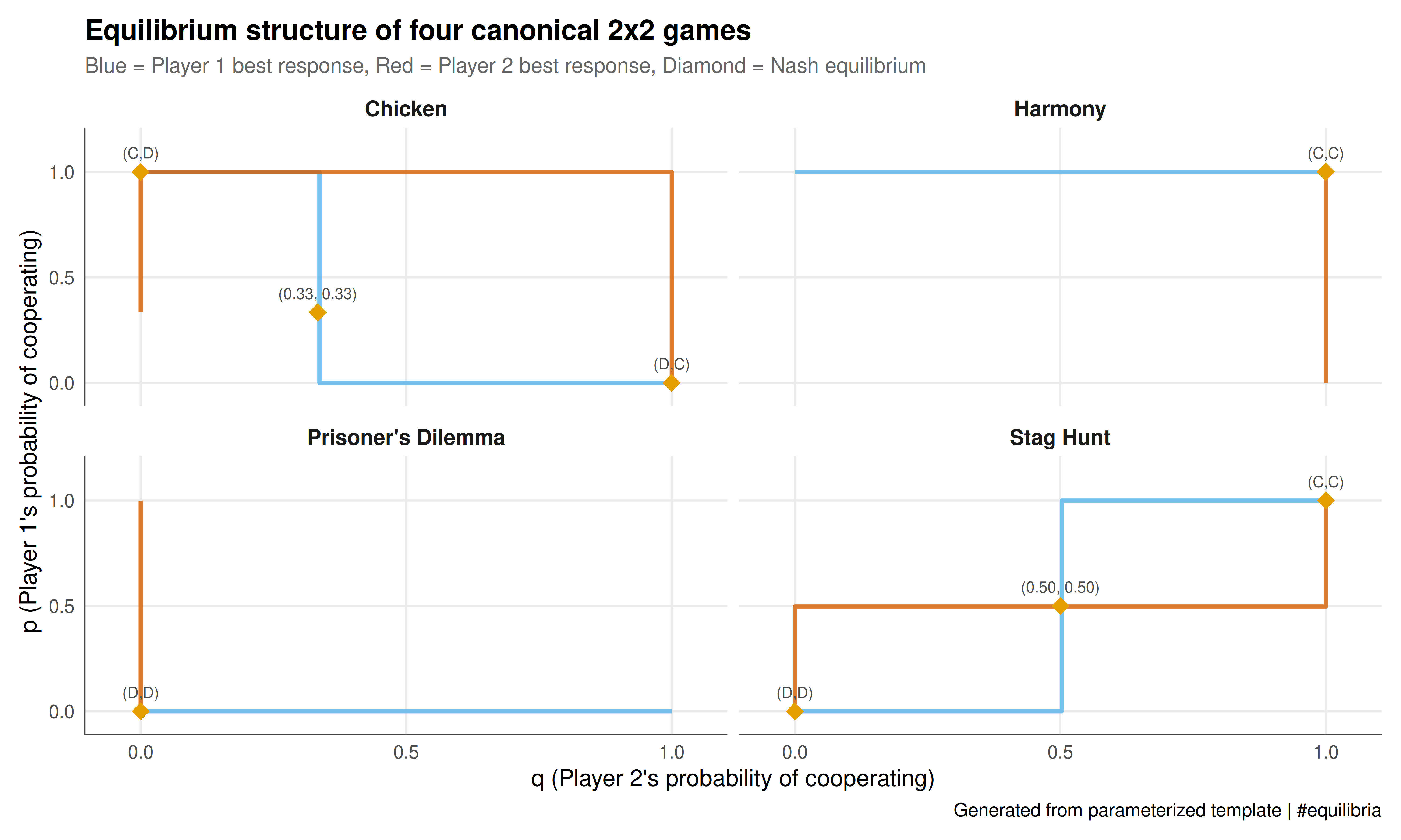
The figure displays the equilibrium structure of all four canonical games in a faceted panel, showing how different parameter values produce different Nash equilibrium configurations. Each panel marks the NE locations in the $(p, q)$ strategy space.
```{r}
#| label: fig-parameterized-games-static
#| fig-cap: "Figure 1. Nash equilibria for four canonical 2x2 games generated from a single parameterized template. Each panel shows the (p, q) strategy space where p is Player 1's probability of cooperating and q is Player 2's. Orange diamonds mark Nash equilibria. The equilibrium structure varies dramatically across games despite the shared analytical framework."
#| dev: [png, pdf]
#| fig-width: 10
#| fig-height: 6
#| dpi: 300
# Build equilibrium point data for all games
eq_points <- do.call(rbind, lapply(results, function(res) {
  if (length(res$equilibria) == 0) return(NULL)
  do.call(rbind, lapply(res$equilibria, function(eq) {
    data.frame(
      game = res$name,
      type = res$type,
      p = eq$p, q = eq$q,
      label = eq$label,
      eq_type = eq$type,
      stringsAsFactors = FALSE
    )
  }))
}))

# Build best-response correspondence data
br_all <- do.call(rbind, lapply(results, function(res) {
  data.frame(
    game = res$name,
    q_axis = res$br_data$q,
    br1_p = res$br_data$br1_p,
    p_axis = res$br_data$p,
    br2_q = res$br_data$br2_q,
    stringsAsFactors = FALSE
  )
}))

# Build payoff label for subtitle
payoff_labels <- sapply(results, function(res) {
  sprintf("%s: R=%d, T=%d, S=%d, P=%d",
          res$name, res$payoffs["R"], res$payoffs["T"],
          res$payoffs["S"], res$payoffs["P"])
})

p_static <- ggplot() +
  # Player 1's best response (p as function of q)
  geom_step(data = br_all,
            aes(x = q_axis, y = br1_p),
            color = okabe_ito[2], linewidth = 1, alpha = 0.8) +
  # Player 2's best response (q as function of p) — swap axes
  geom_step(data = br_all,
            aes(x = br2_q, y = p_axis),
            color = okabe_ito[6], linewidth = 1, alpha = 0.8) +
  # Equilibrium points
  geom_point(data = eq_points,
             aes(x = q, y = p),
             color = okabe_ito[1], size = 4, shape = 18) +
  geom_text(data = eq_points,
            aes(x = q, y = p, label = label),
            vjust = -1.2, size = 2.8, color = "grey30") +
  facet_wrap(~ game, nrow = 2) +
  scale_x_continuous(limits = c(-0.05, 1.05), breaks = c(0, 0.5, 1)) +
  scale_y_continuous(limits = c(-0.05, 1.15), breaks = c(0, 0.5, 1)) +
  labs(
    title = "Equilibrium structure of four canonical 2x2 games",
    subtitle = "Blue = Player 1 best response, Red = Player 2 best response, Diamond = Nash equilibrium",
    x = "q (Player 2's probability of cooperating)",
    y = "p (Player 1's probability of cooperating)",
    caption = "Generated from parameterized template | #equilibria"
  ) +
  theme_publication() +
  theme(strip.text = element_text(size = 11, face = "bold"))

p_static
```
## Interactive figure
The interactive version lets you hover over equilibrium points to see their coordinates and type, and explore the best-response correspondences.
```{r}
#| label: fig-parameterized-games-interactive
eq_points_hover <- eq_points |>
  mutate(hover_text = sprintf("Game: %s\nType: %s\nNE: %s\np=%.2f, q=%.2f",
                               game, type, label, p, q))

p_int <- ggplot() +
  geom_step(data = br_all,
            aes(x = q_axis, y = br1_p,
                text = sprintf("Player 1 BR\nq=%.2f -> p*=%.2f", q_axis, br1_p)),
            color = okabe_ito[2], linewidth = 0.7, alpha = 0.7) +
  geom_step(data = br_all,
            aes(x = br2_q, y = p_axis,
                text = sprintf("Player 2 BR\np=%.2f -> q*=%.2f", p_axis, br2_q)),
            color = okabe_ito[6], linewidth = 0.7, alpha = 0.7) +
  geom_point(data = eq_points_hover,
             aes(x = q, y = p, text = hover_text),
             color = okabe_ito[1], size = 4, shape = 18) +
  facet_wrap(~ game, nrow = 2) +
  scale_x_continuous(limits = c(-0.05, 1.05)) +
  scale_y_continuous(limits = c(-0.05, 1.15)) +
  labs(
    title = "Interactive: equilibria across game types",
    x = "q (Player 2)", y = "p (Player 1)"
  ) +
  theme_publication()

ggplotly(p_int, tooltip = "text") |>
  config(displaylogo = FALSE,
         modeBarButtonsToRemove = c("select2d", "lasso2d", "autoScale2d"))
```
## Interpretation
The four-panel comparison vividly demonstrates how small changes in payoff parameters produce qualitatively different strategic landscapes. In the Prisoner's Dilemma ($T > R > P > S$), the best-response correspondences intersect only at $(p, q) = (0, 0)$: mutual defection is the unique equilibrium regardless of what the other player does. This is the hallmark of a dominant-strategy equilibrium --- the best response is constant.
The Stag Hunt ($R > T > P > S$) has two pure-strategy equilibria --- mutual cooperation and mutual defection --- plus a mixed equilibrium. The mixed equilibrium acts as a coordination threshold: if you believe your opponent cooperates with probability above the threshold, your best response is to cooperate; below the threshold, defect. This captures the fundamental tension in coordination problems where both outcomes are equilibria but one (mutual cooperation) Pareto-dominates the other.
Chicken ($T > R > S > P$) also has three equilibria, but the structure is different. The two pure equilibria are asymmetric (one player swerves, the other goes straight), and the mixed equilibrium involves both players randomising. This is the classic anti-coordination game, where matching actions is the worst outcome, not the best.
Harmony ($R > T > S > P$) has the simplest structure: mutual cooperation is the unique equilibrium and is also the socially optimal outcome. There is no strategic tension --- cooperation is both individually and collectively rational.
For reproducibility, the key advantage of the parameterized approach is that all four analyses share identical code. If we discover a bug in the equilibrium computation or want to improve the visualisation, a single edit propagates to all rendered reports. This is dramatically more maintainable than four separate documents, and it makes the comparative analysis trustworthy: any differences in the output are guaranteed to arise from parameter differences, not from inadvertent code differences.
The batch rendering approach shown in the code section scales to systematic comparative statics. For instance, one could generate 100 reports varying the temptation payoff $T$ from 1 to 10 in steps of 0.1, creating an animation-like sequence that shows exactly when the equilibrium structure transitions from one type to another. This is a powerful pedagogical tool for building intuition about the topology of game spaces.
## Extensions & related tutorials
Parameterized reports are a foundational tool for reproducible game-theoretic research. The approach demonstrated here for $2 \times 2$ games generalises to any analysis where the core logic is stable but the inputs vary.
- [Reproducible game theory workflow](../../reproducibility-open-science/reproducible-game-theory-workflow/) --- integrate parameterized reports into a full Make/targets pipeline
- [Testing game theory code with testthat](../../r-package-development/testing-game-theory-code/) --- validate the analysis engine that powers your parameterized reports
- [Bootstrap inference for game-theoretic quantities](../../statistical-foundations/bootstrap-game-theory/) --- parameterize bootstrap analyses by sample size, number of replications, and confidence level
- [Privacy as a game --- strategic information disclosure](../../ethics-applications/privacy-game-theory/) --- apply parameterized analysis to vary regulation regimes
## References
::: {#refs}
:::