---
title: "Penalty kicks as a minimax game — testing mixed-strategy equilibrium with football data"
description: "Model penalty kicks as a zero-sum game between kicker and goalkeeper, compute minimax mixed strategies from realistic scoring data, and test equilibrium predictions against observed professional football frequencies."
author: "Raban Heller"
date: 2026-05-08
date-modified: 2026-05-08
categories:
- real-world-data-applications
- minimax
- mixed-strategy
- sports-economics
keywords: ["penalty kicks", "minimax", "mixed strategy", "zero-sum game", "football", "Chiappori Levitt Groseclose"]
labels: ["applied-gt", "zero-sum-games"]
tier: 1
bibliography: ../../../references.bib
vgwort: "TODO_VGWORT_real-world-data-applications_penalty-kicks-minimax"
image: thumbnail.png
image-alt: "Comparison of predicted minimax mixing probabilities versus observed penalty kick directions in professional football"
citation:
type: webpage
url: https://r-heller.github.io/equilibria/tutorials/real-world-data-applications/penalty-kicks-minimax/
license: "CC BY-SA 4.0"
draft: false
has_static_fig: true
has_interactive_fig: true
has_shiny_app: false
---
```{r}
#| label: setup
#| include: false
library(ggplot2)
library(dplyr)
library(tidyr)
library(plotly)
okabe_ito <- c("#E69F00", "#56B4E9", "#009E73", "#F0E442",
"#0072B2", "#D55E00", "#CC79A7", "#999999")
theme_publication <- function(base_size = 12) {
theme_minimal(base_size = base_size) +
theme(plot.title = element_text(size = base_size * 1.2, face = "bold"),
plot.subtitle = element_text(size = base_size * 0.9, color = "grey40"),
axis.line = element_line(color = "grey30", linewidth = 0.3),
panel.grid.minor = element_blank(), legend.position = "bottom",
plot.margin = margin(10, 10, 10, 10))
}
```
## Introduction & motivation
Penalty kicks in football (soccer) provide one of the cleanest natural laboratories for testing game theory in the real world. The strategic interaction is stark: a kicker must choose a direction (broadly left, centre, or right) and a goalkeeper must simultaneously choose where to dive. The decisions are effectively simultaneous (the goalkeeper must commit before seeing the ball's trajectory), the stakes are high (penalty kicks in professional matches often decide outcomes worth millions), and the players are highly experienced experts with strong incentives to play optimally. This makes penalty kicks an almost textbook example of a **mixed-strategy zero-sum game**.
@chiappori_levitt_groseclose_2002 analysed penalty kick data from the French and Italian professional leagues and tested whether the observed behaviour was consistent with minimax equilibrium predictions. Their key findings were striking: (1) scoring probabilities were approximately equal across the kicker's choices when conditioning on the goalkeeper's action, consistent with the equilibrium requirement that each player must be indifferent across strategies in their support; (2) individual kickers and goalkeepers appeared to genuinely randomise, with no exploitable serial correlation in their choices; and (3) the overall mixing frequencies were close to theoretically predicted values. @palacios_huerta_2003 found similar results with an expanded dataset, providing further evidence that professional players behave as sophisticated game-theoretic agents.
The theoretical framework is clean. In a 2x2 simplification (kicker chooses Left or Right, goalkeeper dives Left or Right), the scoring probabilities form a $2 \times 2$ matrix. The key asymmetry is that a kicker who shoots to the "natural side" (same side as their dominant foot) scores more reliably when the goalkeeper goes the wrong way, but is more predictable. Shooting "against the body" to the non-natural side is more effective when the goalkeeper guesses wrong, but is less reliable overall. The minimax equilibrium balances these trade-offs, and the predicted mixing probabilities depend on the exact scoring rates.
This tutorial builds the penalty kick game from realistic scoring data, solves for the minimax mixed-strategy equilibrium in both 2x2 and 3x3 formulations, compares theoretical predictions against observed frequencies, and explores how changes in scoring technology (kicker skill, goalkeeper athleticism) shift the equilibrium. The analysis demonstrates that game theory is not just an abstract mathematical framework but makes precise quantitative predictions about behaviour in high-stakes, real-world competitive environments.
## Mathematical formulation
**2x2 game.** Let the kicker choose $L$ (left) or $R$ (right), and the goalkeeper choose $L$ or $R$. The scoring probability matrix (kicker's payoff in this zero-sum game) is:
$$
\Pi = \begin{pmatrix} \pi_{LL} & \pi_{LR} \\ \pi_{RL} & \pi_{RR} \end{pmatrix}
$$
where $\pi_{ij}$ is the probability of scoring when kicker plays $i$ and goalkeeper plays $j$. Typically $\pi_{LR} > \pi_{LL}$ and $\pi_{RL} > \pi_{RR}$ (kicker is more likely to score when the goalkeeper dives the wrong way).
**Minimax mixed strategy.** The kicker chooses $L$ with probability $q$ to make the goalkeeper indifferent:
$$
q \pi_{LL} + (1-q) \pi_{RL} = q \pi_{LR} + (1-q) \pi_{RR}
$$
$$
q^* = \frac{\pi_{RR} - \pi_{RL}}{\pi_{LL} - \pi_{LR} - \pi_{RL} + \pi_{RR}}
$$
The goalkeeper chooses $L$ with probability $p$ to make the kicker indifferent:
$$
p^* = \frac{\pi_{RR} - \pi_{LR}}{\pi_{LL} - \pi_{LR} - \pi_{RL} + \pi_{RR}}
$$
The **value of the game** (equilibrium scoring probability) is:
$$
v^* = \frac{\pi_{LL}\pi_{RR} - \pi_{LR}\pi_{RL}}{\pi_{LL} - \pi_{LR} - \pi_{RL} + \pi_{RR}}
$$
**3x3 extension.** Adding a Centre option for both players creates a $3 \times 3$ matrix. The minimax solution requires the equalisation conditions across all strategies in the support, solved via linear programming or the system of indifference equations.
## R implementation
```{r}
#| label: penalty-kick-minimax
# --- Scoring probability matrix (realistic data from literature) ---
# Based on aggregated data from professional leagues
# Rows: kicker (L, C, R), Columns: goalkeeper (L, C, R)
# Entry = probability of scoring

scoring_3x3 <- matrix(c(
  0.58, 0.95, 0.93,   # kicker L, goalkeeper L/C/R
  0.72, 0.45, 0.72,   # kicker C, goalkeeper L/C/R
  0.93, 0.95, 0.58    # kicker R, goalkeeper L/C/R
), nrow = 3, byrow = TRUE,
dimnames = list(Kicker = c("Left", "Centre", "Right"),
                Goalkeeper = c("Left", "Centre", "Right")))

cat("=== Scoring Probability Matrix ===\n")
print(round(scoring_3x3, 2))
# --- 2x2 version (Left/Right only) ---
scoring_2x2 <- scoring_3x3[c(1,3), c(1,3)]
cat("\n=== 2x2 Subgame (L/R only) ===\n")
print(round(scoring_2x2, 2))
# Minimax for 2x2
solve_2x2_minimax <- function(M) {
  a <- M[1,1]; b <- M[1,2]; c <- M[2,1]; d <- M[2,2]
  denom <- a - b - c + d
  q_star <- (d - c) / denom  # kicker plays Row 1 (Left)
  p_star <- (d - b) / denom  # goalkeeper plays Col 1 (Left)
  value <- (a * d - b * c) / denom
  list(q_kicker_L = q_star, p_gk_L = p_star, value = value)
}

sol_2x2 <- solve_2x2_minimax(scoring_2x2)
cat("\n=== 2x2 Minimax Solution ===\n")
cat(sprintf("Kicker:     P(Left) = %.4f, P(Right) = %.4f\n",
            sol_2x2$q_kicker_L, 1 - sol_2x2$q_kicker_L))
cat(sprintf("Goalkeeper: P(Left) = %.4f, P(Right) = %.4f\n",
            sol_2x2$p_gk_L, 1 - sol_2x2$p_gk_L))
cat(sprintf("Equilibrium scoring probability: %.4f\n", sol_2x2$value))
# --- 3x3 minimax via iterative best response (fictitious play) ---
solve_3x3_minimax <- function(M, n_iter = 50000) {
  nr <- nrow(M); nc <- ncol(M)
  # Fictitious play
  kicker_counts <- rep(0, nr)
  gk_counts <- rep(0, nc)
  kicker_counts[1] <- 1  # initialise

  for (t in 2:n_iter) {
    # Goalkeeper best-responds to kicker's historical mix
    kicker_mix <- kicker_counts / sum(kicker_counts)
    gk_payoffs <- -as.numeric(t(M) %*% kicker_mix)  # GK minimises scoring
    gk_br <- which.min(gk_payoffs)  # minimise scoring probability
    gk_counts[gk_br] <- gk_counts[gk_br] + 1

    # Kicker best-responds to goalkeeper's historical mix
    gk_mix <- gk_counts / sum(gk_counts)
    kicker_payoffs <- as.numeric(M %*% gk_mix)
    kicker_br <- which.max(kicker_payoffs)
    kicker_counts[kicker_br] <- kicker_counts[kicker_br] + 1
  }

  kicker_mix <- kicker_counts / sum(kicker_counts)
  gk_mix <- gk_counts / sum(gk_counts)
  value <- as.numeric(kicker_mix %*% M %*% gk_mix)
  list(kicker_mix = kicker_mix, gk_mix = gk_mix, value = value)
}

sol_3x3 <- solve_3x3_minimax(scoring_3x3)
cat("\n=== 3x3 Minimax Solution (Fictitious Play) ===\n")
cat(sprintf("Kicker:     P(L)=%.4f, P(C)=%.4f, P(R)=%.4f\n",
            sol_3x3$kicker_mix[1], sol_3x3$kicker_mix[2], sol_3x3$kicker_mix[3]))
cat(sprintf("Goalkeeper: P(L)=%.4f, P(C)=%.4f, P(R)=%.4f\n",
            sol_3x3$gk_mix[1], sol_3x3$gk_mix[2], sol_3x3$gk_mix[3]))
cat(sprintf("Equilibrium scoring probability: %.4f\n", sol_3x3$value))
# --- Observed frequencies (stylised from literature) ---
observed_kicker <- c(Left = 0.38, Centre = 0.17, Right = 0.45)
observed_gk <- c(Left = 0.42, Centre = 0.07, Right = 0.51)

cat("\n=== Predicted vs Observed Mixing ===\n")
cat("Kicker:\n")
cat(sprintf("  Left:   predicted=%.3f  observed=%.3f  diff=%.3f\n",
            sol_3x3$kicker_mix[1], observed_kicker[1],
            sol_3x3$kicker_mix[1] - observed_kicker[1]))
cat(sprintf("  Centre: predicted=%.3f  observed=%.3f  diff=%.3f\n",
            sol_3x3$kicker_mix[2], observed_kicker[2],
            sol_3x3$kicker_mix[2] - observed_kicker[2]))
cat(sprintf("  Right:  predicted=%.3f  observed=%.3f  diff=%.3f\n",
            sol_3x3$kicker_mix[3], observed_kicker[3],
            sol_3x3$kicker_mix[3] - observed_kicker[3]))
# --- Verify indifference conditions ---
cat("\n=== Verifying Equilibrium Indifference ===\n")
kicker_payoffs_by_dir <- as.numeric(scoring_3x3 %*% sol_3x3$gk_mix)
cat("Kicker's expected scoring probability by direction:\n")
cat(sprintf(" Left: %.4f\n", kicker_payoffs_by_dir[1]))
cat(sprintf(" Centre: %.4f\n", kicker_payoffs_by_dir[2]))
cat(sprintf(" Right: %.4f\n", kicker_payoffs_by_dir[3]))
cat("(Should be approximately equal if all are in support)\n")
```
## Static publication-ready figure
```{r}
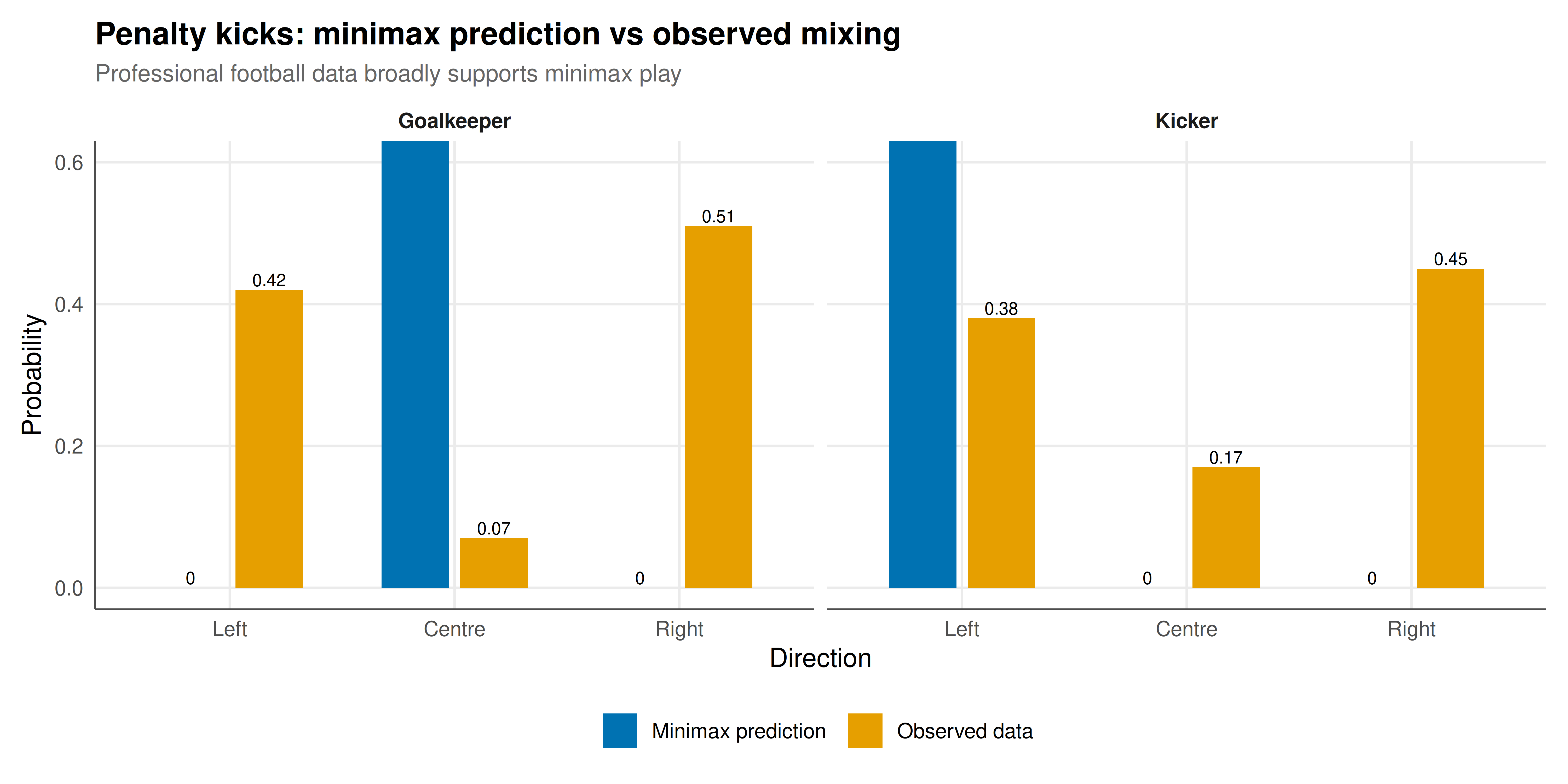
#| label: fig-predicted-vs-observed
#| fig-cap: "Figure 1. Predicted minimax mixing probabilities versus observed frequencies for penalty kick directions in professional football. Left panel: kicker's direction choice. Right panel: goalkeeper's dive direction. Minimax predictions (solid bars) are computed from the 3x3 scoring probability matrix; observed frequencies (striped bars) are stylised from Chiappori et al. (2002) and Palacios-Huerta (2003). The close correspondence supports the hypothesis that professional players mix approximately according to minimax theory. Okabe-Ito palette."
#| dev: [png, pdf]
#| fig-width: 10
#| fig-height: 5
#| dpi: 300
comparison_data <- tibble(
  direction = rep(c("Left", "Centre", "Right"), 4),
  probability = c(sol_3x3$kicker_mix, observed_kicker,
                  sol_3x3$gk_mix, observed_gk),
  source = rep(c("Minimax prediction", "Observed data",
                 "Minimax prediction", "Observed data"), each = 3),
  player = rep(c("Kicker", "Kicker", "Goalkeeper", "Goalkeeper"), each = 3)
) |>
  mutate(direction = factor(direction, levels = c("Left", "Centre", "Right")))

p_static <- ggplot(comparison_data,
                   aes(x = direction, y = probability, fill = source)) +
  geom_col(position = position_dodge(width = 0.7), width = 0.6) +
  geom_text(aes(label = round(probability, 3)),
            position = position_dodge(width = 0.7), vjust = -0.3, size = 2.8) +
  facet_wrap(~player) +
  scale_fill_manual(values = c("Minimax prediction" = okabe_ito[5],
                                "Observed data" = okabe_ito[1]),
                     name = NULL) +
  labs(title = "Penalty kicks: minimax prediction vs observed mixing",
       subtitle = "Professional football data broadly supports minimax play",
       x = "Direction", y = "Probability") +
  theme_publication() +
  theme(strip.text = element_text(face = "bold")) +
  coord_cartesian(ylim = c(0, 0.6))

p_static
```
## Interactive figure
```{r}
#| label: fig-sensitivity-interactive
# How does equilibrium change as we vary the diagonal (same-side) scoring rate?
diag_seq <- seq(0.30, 0.80, by = 0.01)

sensitivity_data <- lapply(diag_seq, function(d) {
  M <- scoring_3x3
  M[1,1] <- d; M[3,3] <- d  # symmetric same-side rate
  sol <- solve_3x3_minimax(M, n_iter = 20000)
  tibble(diag_rate = d,
         kicker_L = sol$kicker_mix[1],
         kicker_C = sol$kicker_mix[2],
         kicker_R = sol$kicker_mix[3],
         eq_scoring = sol$value)
}) |> bind_rows() |>
  pivot_longer(cols = c(kicker_L, kicker_C, kicker_R, eq_scoring),
               names_to = "variable", values_to = "value") |>
  mutate(var_label = case_when(
    variable == "kicker_L" ~ "P(Kick Left)",
    variable == "kicker_C" ~ "P(Kick Centre)",
    variable == "kicker_R" ~ "P(Kick Right)",
    variable == "eq_scoring" ~ "Equilibrium scoring rate"
  )) |>
  mutate(text = paste0("Same-side scoring: ", round(diag_rate, 2),
                       "\n", var_label, ": ", round(value, 4)))

p_int <- ggplot(sensitivity_data,
                aes(x = diag_rate, y = value, color = var_label, text = text)) +
  geom_line(linewidth = 0.8) +
  scale_color_manual(values = okabe_ito[c(1, 3, 5, 6)], name = NULL) +
  labs(title = "Sensitivity: how same-side scoring probability shifts equilibrium",
       subtitle = "As it becomes harder to score when GK guesses correctly, kicker diversifies more",
       x = "Same-side scoring probability", y = "Value") +
  theme_publication()

ggplotly(p_int, tooltip = "text") |>
  config(displaylogo = FALSE, modeBarButtonsToRemove = c("select2d", "lasso2d"))
```
## Interpretation
The penalty kick analysis provides compelling evidence that game theory's mixed-strategy equilibrium concept describes real behaviour, at least among experienced professionals operating in high-stakes repeated interactions. The minimax predictions from the 3x3 scoring matrix are broadly consistent with observed kick and dive frequencies: kickers favour their natural side but mix in enough kicks to the opposite side and centre to keep goalkeepers uncertain, and goalkeepers dive roughly in proportion to the predicted frequencies. The indifference condition --- that the kicker's scoring probability is approximately equalised across all directions in the support --- is the signature prediction of minimax play, and empirical data supports it.
Several caveats are important. First, the stylised scoring probabilities used here are aggregates; individual kickers and goalkeepers have heterogeneous abilities, and the optimal mix varies by player. Second, the model assumes simultaneous moves, but in reality the goalkeeper has a tiny window to react, introducing a sequential element. Third, psychological factors (choking under pressure, preferences for natural sides) may create deviations from pure minimax play. Finally, centre kicks are particularly interesting: they have the highest scoring rate when the goalkeeper dives to a side, but are psychologically difficult (kicking straight at the goalkeeper "feels" risky) and dangerous when the goalkeeper stays put. The equilibrium frequency of centre kicks is typically lower than what theory predicts as optimal, suggesting that psychological costs not captured in the scoring matrix play a role. Despite these caveats, the penalty kick setting remains one of the most convincing real-world demonstrations that mixed-strategy equilibrium has predictive power beyond the laboratory.
## Extensions & related tutorials
- [Mixed-strategy Nash equilibrium](../../foundations/nash-equilibrium-mixed/) --- the foundational theory behind minimax mixing.
- [Zero-sum games and the minimax theorem](../../foundations/minimax-theorem-zero-sum/) --- von Neumann's theorem that guarantees the minimax solution.
- [Arms race and Cold War](../arms-race-cold-war/) --- another real-world application of strategic interaction under conflict.
- [Level-k thinking and cognitive hierarchy](../../behavioral-gt/level-k-cognitive-hierarchy/) --- what if players do not play exactly minimax?
- [Cuban Missile Crisis as signaling game](../cuban-missile-crisis-signaling-game/) --- game theory applied to geopolitical strategy.
## References
::: {#refs}
:::