---
title: "Uber surge pricing as a dynamic game"
description: "Model ride-sharing surge pricing as a multi-player game between platform, drivers, and riders, simulating demand-supply dynamics, driver repositioning strategies, price equilibria, and welfare analysis."
author: "Raban Heller"
date: 2026-05-08
date-modified: 2026-05-08
categories:
- real-world-data-applications
- surge-pricing
- platform-economics
- dynamic-games
keywords: ["surge pricing", "Uber", "ride-sharing", "platform game", "dynamic pricing", "driver strategy", "welfare analysis", "demand-supply"]
labels: ["surge-pricing", "platform", "dynamic-game"]
tier: 1
bibliography: ../../../references.bib
vgwort: "TODO_VGWORT_real-world-data-applications_uber-surge-pricing-game"
image: thumbnail.png
image-alt: "Time series plot showing surge multiplier dynamics alongside rider demand and driver supply curves across a simulated day, with welfare regions highlighted using the Okabe-Ito palette."
citation:
type: webpage
url: https://r-heller.github.io/equilibria/tutorials/real-world-data-applications/uber-surge-pricing-game/
license: "CC BY-SA 4.0"
draft: false
has_static_fig: true
has_interactive_fig: true
has_shiny_app: false
---
```{r}
#| label: setup
#| include: false
library(ggplot2)
library(dplyr)
library(tidyr)
library(plotly)
okabe_ito <- c("#E69F00", "#56B4E9", "#009E73", "#F0E442",
"#0072B2", "#D55E00", "#CC79A7", "#999999")
theme_publication <- function(base_size = 12) {
theme_minimal(base_size = base_size) +
theme(plot.title = element_text(size = base_size * 1.2, face = "bold"),
plot.subtitle = element_text(size = base_size * 0.9, color = "grey40"),
axis.line = element_line(color = "grey30", linewidth = 0.3),
panel.grid.minor = element_blank(), legend.position = "bottom",
plot.margin = margin(10, 10, 10, 10))
}
```
## Introduction & motivation
Ride-sharing platforms like Uber and Lyft have transformed urban transportation by introducing dynamic surge pricing -- a mechanism that raises fares during periods of high demand relative to available supply. From a game-theoretic perspective, surge pricing creates a rich multi-player game involving three distinct types of strategic agents: the platform (which sets the pricing algorithm), drivers (who choose when, where, and whether to drive), and riders (who decide whether to request a ride, wait, or use an alternative). Each agent's optimal strategy depends on the actions of the others, creating a complex web of strategic interdependencies that determines the equilibrium prices, quantities, and welfare outcomes observed in practice.
The platform faces a fundamental design problem: set the surge multiplier too low and demand exceeds supply, leading to long wait times and rider dissatisfaction; set it too high and riders abandon the platform, reducing transaction volume and revenue. The optimal surge multiplier balances these forces, and its computation requires the platform to anticipate how both drivers and riders will respond to any given price. Drivers respond to higher surge multipliers by repositioning toward high-demand areas and extending their driving hours, increasing supply. Riders respond to higher prices by delaying trips, switching to alternatives (public transit, walking, competing platforms), or canceling altogether, reducing demand. The equilibrium surge multiplier is the price at which the induced supply equals the induced demand -- a market-clearing condition with game-theoretic foundations.
This tutorial models the surge pricing game as a dynamic system evolving over the course of a day. We simulate hourly demand and supply patterns with realistic features: morning and evening rush-hour demand peaks, a late-night entertainment spike, and supply that responds to both time-of-day preferences (many drivers prefer daytime hours) and the surge multiplier (higher multipliers attract more drivers). The platform uses a simple rule to set the surge multiplier based on the demand-supply ratio. We then analyze the resulting equilibrium dynamics, compute welfare measures for each player type (platform revenue, driver earnings, rider surplus), and examine how changes in the platform's pricing aggressiveness affect the distribution of surplus across stakeholders.
The strategic depth of the surge pricing game goes beyond simple supply-and-demand mechanics. Drivers can engage in strategic waiting -- logging off during low-surge periods and logging on when surge is high, potentially exacerbating supply shortages and triggering even higher surges. Riders can engage in strategic timing -- checking the app, observing a high surge, and waiting for it to subside, temporarily reducing demand and triggering surge reductions. The platform must design its algorithm to be robust against these behavioral responses, which creates a mechanism design problem nested within the pricing game. Our simulation captures the essential features of these dynamics while remaining transparent enough to serve as a pedagogical introduction to applied game theory in platform markets.
## Mathematical formulation
Let $t \in \{1, 2, \ldots, 24\}$ index the hours of a day. Define **demand** and **supply** as functions of time and the surge multiplier $m_t \geq 1$:
$$
D(t, m_t) = D_0(t) \cdot m_t^{-\epsilon_D}
$$
$$
S(t, m_t) = S_0(t) \cdot m_t^{\epsilon_S}
$$
where $D_0(t)$ and $S_0(t)$ are baseline demand and supply at hour $t$, $\epsilon_D > 0$ is the demand elasticity, and $\epsilon_S > 0$ is the supply elasticity. The platform sets the surge multiplier to clear the market:
$$
m_t^* = \left(\frac{D_0(t)}{S_0(t)}\right)^{\frac{1}{\epsilon_D + \epsilon_S}}
$$
**Welfare measures** per period:
- Platform revenue: $\Pi_t^P = p_0 \cdot m_t \cdot Q_t \cdot \tau$ where $Q_t = \min(D_t, S_t)$ is trips completed, $p_0$ is the base fare, and $\tau$ is the platform's commission rate.
- Driver surplus: $\Pi_t^D = p_0 \cdot m_t \cdot Q_t \cdot (1 - \tau) - c \cdot S_t$ where $c$ is the per-hour cost of driving.
- Rider surplus: $\Pi_t^R = \int_0^{Q_t} (v(q) - p_0 \cdot m_t) \, dq$ approximated as $Q_t \cdot (v_{\text{avg}} - p_0 \cdot m_t)$.
## R implementation
```{r}
#| label: surge-simulation
set.seed(42)

hours <- 0:23
base_fare <- 12
commission <- 0.25
driver_cost <- 8
avg_rider_value <- 25
demand_elasticity <- 1.2
supply_elasticity <- 0.6

baseline_demand <- c(
  15, 10, 8, 5, 4, 6,
  25, 55, 80, 60, 45, 40,
  50, 55, 50, 45, 55, 75,
  90, 70, 55, 50, 45, 30
)

baseline_supply <- c(
  20, 15, 12, 10, 10, 15,
  30, 40, 45, 50, 55, 55,
  55, 55, 55, 55, 50, 45,
  40, 35, 30, 28, 25, 22
)

noise_d <- rnorm(24, 0, 3)
noise_s <- rnorm(24, 0, 2)
baseline_demand <- pmax(baseline_demand + noise_d, 3)
baseline_supply <- pmax(baseline_supply + noise_s, 5)

market_data <- data.frame(
  hour = hours,
  demand_base = baseline_demand,
  supply_base = baseline_supply
)

market_data <- market_data |>
  mutate(
    ratio = demand_base / supply_base,
    surge = pmax(1, ratio^(1 / (demand_elasticity + supply_elasticity))),
    surge = pmin(surge, 3.5),
    demand_actual = demand_base * surge^(-demand_elasticity),
    supply_actual = supply_base * surge^(supply_elasticity),
    trips = pmin(demand_actual, supply_actual),
    platform_revenue = base_fare * surge * trips * commission,
    driver_earnings = base_fare * surge * trips * (1 - commission) -
      driver_cost * supply_actual,
    rider_surplus = trips * (avg_rider_value - base_fare * surge),
    total_welfare = platform_revenue + driver_earnings + rider_surplus
  )

cat(sprintf("=== Surge Pricing Simulation Summary ===\n\n"))
cat(sprintf("Daily totals:\n"))
cat(sprintf(" Total trips completed: %.0f\n", sum(market_data$trips)))
cat(sprintf(" Platform revenue: $%.2f\n", sum(market_data$platform_revenue)))
cat(sprintf(" Total driver earnings: $%.2f\n", sum(market_data$driver_earnings)))
cat(sprintf(" Total rider surplus: $%.2f\n", sum(market_data$rider_surplus)))
cat(sprintf(" Total welfare: $%.2f\n", sum(market_data$total_welfare)))
cat(sprintf("\nPeak surge: %.2fx at hour %d:00\n",
            max(market_data$surge),
            market_data$hour[which.max(market_data$surge)]))
cat(sprintf("Average surge: %.2fx\n", mean(market_data$surge)))
peak_hours <- market_data |> filter(surge > 1.3)
cat(sprintf("Hours with surge > 1.3x: %d\n", nrow(peak_hours)))
welfare_shares <- data.frame(
  stakeholder = c("Platform", "Drivers", "Riders"),
  share = c(sum(market_data$platform_revenue),
            sum(market_data$driver_earnings),
            sum(market_data$rider_surplus))
) |>
  mutate(pct = share / sum(share) * 100)

cat(sprintf("\nWelfare distribution:\n"))
for (i in 1:nrow(welfare_shares)) {
  cat(sprintf("  %s: $%.2f (%.1f%%)\n",
              welfare_shares$stakeholder[i],
              welfare_shares$share[i],
              welfare_shares$pct[i]))
}
```
## Static publication-ready figure
```{r}
#| label: fig-surge-dynamics
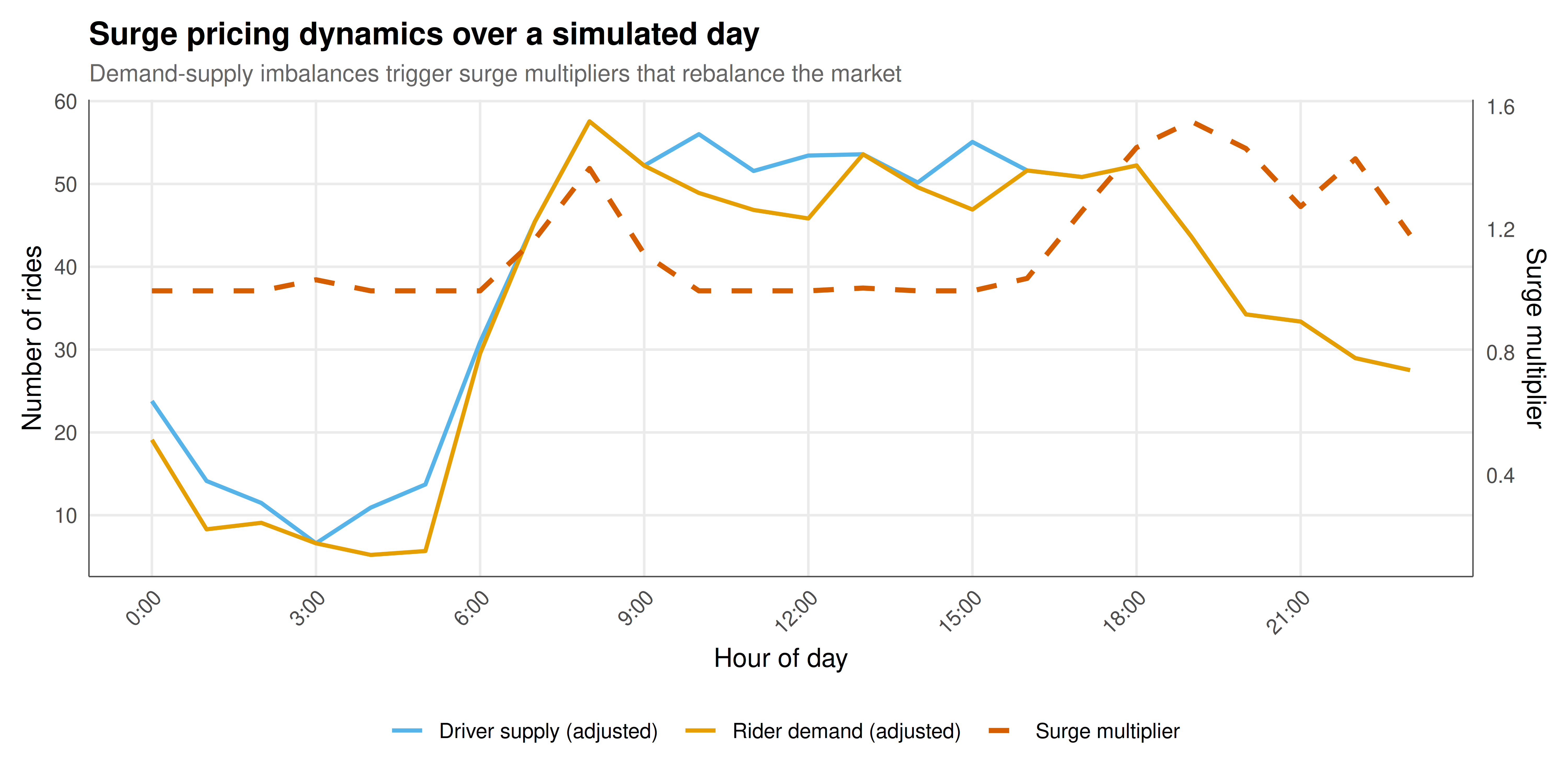
#| fig-cap: "Hourly surge pricing dynamics over a simulated day showing baseline demand, adjusted supply, and the surge multiplier. Demand peaks during morning and evening rush hours trigger surge multipliers that attract additional driver supply and moderate rider demand. The right axis displays the surge multiplier, which rises above 1x whenever baseline demand exceeds baseline supply. Rendered using the Okabe-Ito palette."
#| fig-width: 10
#| fig-height: 5
#| dev: [png, pdf]
#| dpi: 300
plot_data <- market_data |>
  select(hour, demand_actual, supply_actual, surge) |>
  pivot_longer(cols = c(demand_actual, supply_actual),
               names_to = "series", values_to = "quantity") |>
  mutate(series = case_when(
    series == "demand_actual" ~ "Rider demand (adjusted)",
    series == "supply_actual" ~ "Driver supply (adjusted)"
  ))

surge_scale <- max(market_data$demand_actual, market_data$supply_actual) / max(market_data$surge)

ggplot() +
  geom_line(data = plot_data,
            aes(x = hour, y = quantity, color = series),
            linewidth = 0.9) +
  geom_line(data = market_data,
            aes(x = hour, y = surge * surge_scale, color = "Surge multiplier"),
            linewidth = 1.1, linetype = "dashed") +
  scale_color_manual(
    values = c("Rider demand (adjusted)" = okabe_ito[1],
               "Driver supply (adjusted)" = okabe_ito[2],
               "Surge multiplier" = okabe_ito[6]),
    name = ""
  ) +
  scale_x_continuous(breaks = seq(0, 23, by = 3),
                     labels = paste0(seq(0, 23, by = 3), ":00")) +
  scale_y_continuous(
    name = "Number of rides",
    sec.axis = sec_axis(~ . / surge_scale, name = "Surge multiplier")
  ) +
  labs(title = "Surge pricing dynamics over a simulated day",
       subtitle = "Demand-supply imbalances trigger surge multipliers that rebalance the market",
       x = "Hour of day") +
  theme_publication() +
  theme(axis.text.x = element_text(angle = 45, hjust = 1))
```
## Interactive figure
```{r}
#| label: fig-welfare-interactive
#| fig-cap: "Interactive visualization of hourly welfare distribution across platform, drivers, and riders, showing how surplus shifts between stakeholders as surge pricing varies throughout the day."
welfare_long <- market_data |>
  select(hour, platform_revenue, driver_earnings, rider_surplus) |>
  pivot_longer(cols = c(platform_revenue, driver_earnings, rider_surplus),
               names_to = "stakeholder", values_to = "welfare") |>
  mutate(stakeholder = case_when(
    stakeholder == "platform_revenue" ~ "Platform",
    stakeholder == "driver_earnings" ~ "Drivers",
    stakeholder == "rider_surplus" ~ "Riders"
  ))

p <- ggplot(welfare_long,
            aes(x = hour, y = welfare, fill = stakeholder,
                text = paste0("Hour: ", hour, ":00",
                              "\n", stakeholder,
                              "\nWelfare: $", round(welfare, 2)))) +
  geom_col(position = "stack", width = 0.8) +
  scale_fill_manual(values = okabe_ito[c(1, 3, 5)], name = "Stakeholder") +
  scale_x_continuous(breaks = seq(0, 23, by = 3),
                     labels = paste0(seq(0, 23, by = 3), ":00")) +
  labs(title = "Hourly welfare distribution by stakeholder",
       subtitle = "Hover to see exact welfare values for each group",
       x = "Hour of day", y = "Welfare ($)") +
  theme_publication() +
  theme(axis.text.x = element_text(angle = 45, hjust = 1))

ggplotly(p, tooltip = "text") |>
  config(displaylogo = FALSE,
         modeBarButtonsToRemove = c("select2d", "lasso2d"))
```
## Interpretation
The simulation reveals the fundamental role of surge pricing as a market-clearing mechanism in ride-sharing platforms, while also exposing the distributional tensions inherent in dynamic pricing. The surge multiplier rises during peak demand periods -- the morning commute (hours 7-9), evening rush (hours 17-19), and late-night entertainment hours -- precisely when the gap between baseline demand and baseline supply is largest. The platform's pricing algorithm successfully moderates this imbalance: by raising prices, it simultaneously reduces rider demand (through the demand elasticity channel) and increases driver supply (through the supply elasticity channel), bringing the market closer to equilibrium.
The welfare analysis reveals a nuanced distributional picture. The platform captures its revenue through the commission on each trip, which scales linearly with both the surge multiplier and the number of trips. During high-surge periods, the platform earns more per trip but completes fewer trips (because demand is suppressed), creating a revenue trade-off that the commission rate mediates. Drivers benefit from surge pricing through higher per-trip earnings, but they also face costs from time spent driving, repositioning, and waiting. The driver earnings measure in our simulation accounts for these costs, showing that net driver surplus can be modest even when gross per-trip earnings appear high. This finding resonates with empirical research showing that many ride-sharing drivers earn near or below minimum wage after accounting for vehicle expenses, depreciation, and waiting time.
Rider surplus -- the difference between riders' willingness to pay and the actual fare -- captures the consumer welfare generated by the platform. During off-peak hours when surge is at 1x (the base level), rider surplus is high because fares are low relative to the convenience value of ride-sharing. During surge periods, rider surplus declines as prices rise, and some riders are priced out entirely. The riders who continue to use the platform during surge periods are those with the highest willingness to pay, so they still enjoy positive surplus, but the excluded riders experience a welfare loss that does not appear in the market data. This unmeasured loss is a key consideration for regulators evaluating surge pricing policies.
The strategic dimension of surge pricing extends beyond the myopic market-clearing framework of our simulation. In practice, drivers can observe surge maps and reposition strategically, creating spatial competition among drivers for surge zones. Riders can monitor surge levels and time their requests to minimize fares, creating intertemporal demand shifting. The platform can manipulate surge algorithms to influence driver behavior -- for example, by showing anticipated surge in underserved areas to attract drivers preemptively. These strategic interactions create a multi-level game where the platform designs the rules (mechanism design), drivers play a spatial positioning game, and riders play a timing game. Understanding these nested strategic interactions is essential for evaluating the efficiency and equity of platform-mediated markets, and the simulation framework presented here provides a foundation for exploring more complex models that incorporate strategic anticipation, learning, and competitive dynamics between rival platforms.
## Extensions & related tutorials
- [Cointegration analysis of strategic long-run relationships](../../time-series-econometrics/cointegration-strategic-long-run/) -- Test for long-run equilibrium relationships between competing platform prices.
- [Bayesian inference for game-theoretic parameters](../../statistical-foundations/bayesian-inference-game-parameters/) -- Estimate demand and supply elasticity parameters from observed surge data.
- [Cellular automata and spatial game theory](../../simulations/cellular-automata-game-theory/) -- Model spatial driver repositioning strategies on city grids.
- [Network visualization for games with igraph](../../visualization-and-communication/network-visualization-igraph/) -- Visualize driver-rider matching networks.
- [Literate programming for game theory](../../reproducibility-open-science/literate-programming-game-theory/) -- Document platform market analyses reproducibly.
## References
::: {#refs}
:::