---
title: "Cellular automata and spatial game theory"
description: "Implement spatial games on lattice grids where agents play the Prisoner's Dilemma with neighbors, exploring strategy invasion dynamics, cluster formation, and the Nowak-May spatial chaos phenomenon."
author: "Raban Heller"
date: 2026-05-08
date-modified: 2026-05-08
categories:
- simulations
- spatial-games
- cellular-automata
- cooperation
keywords: ["cellular automata", "spatial game theory", "Prisoner's Dilemma", "Nowak-May", "cooperation", "lattice", "strategy dynamics"]
labels: ["cellular-automata", "spatial", "simulation"]
tier: 1
bibliography: ../../../references.bib
vgwort: "TODO_VGWORT_simulations_cellular-automata-game-theory"
image: thumbnail.png
image-alt: "Grid heatmap showing spatial distribution of cooperators and defectors on a lattice after evolutionary dynamics, with cluster formation visible, rendered using the Okabe-Ito palette."
citation:
type: webpage
url: https://r-heller.github.io/equilibria/tutorials/simulations/cellular-automata-game-theory/
license: "CC BY-SA 4.0"
draft: false
has_static_fig: true
has_interactive_fig: true
has_shiny_app: false
---
```{r}
#| label: setup
#| include: false
library(ggplot2)
library(dplyr)
library(tidyr)
library(plotly)
okabe_ito <- c("#E69F00", "#56B4E9", "#009E73", "#F0E442",
"#0072B2", "#D55E00", "#CC79A7", "#999999")
theme_publication <- function(base_size = 12) {
theme_minimal(base_size = base_size) +
theme(plot.title = element_text(size = base_size * 1.2, face = "bold"),
plot.subtitle = element_text(size = base_size * 0.9, color = "grey40"),
axis.line = element_line(color = "grey30", linewidth = 0.3),
panel.grid.minor = element_blank(), legend.position = "bottom",
plot.margin = margin(10, 10, 10, 10))
}
```
## Introduction & motivation
The Prisoner's Dilemma is the most studied game in all of game theory, capturing the fundamental tension between individual rationality and collective welfare. In the standard one-shot version, defection strictly dominates cooperation, leading to the unique Nash equilibrium where both players defect -- even though mutual cooperation would be better for both. This pessimistic prediction has motivated decades of research into mechanisms that can sustain cooperation: repeated interactions, reputation, punishment, kin selection, and group selection. Among the most elegant and surprising of these mechanisms is spatial structure, first systematically studied by Nowak and May (1992), who showed that cooperation can persist on a spatial lattice even when players are memoryless, have no ability to punish, and interact only once with each neighbor per round.
In a spatial game, players occupy cells on a grid (typically a two-dimensional square lattice) and interact with their immediate neighbors. Each cell holds a strategy -- cooperate (C) or defect (D) -- and accumulates payoffs from Prisoner's Dilemma interactions with all neighbors. At the end of each round, every cell updates its strategy by imitating the most successful neighbor (including itself). This deterministic, synchronous update rule is the hallmark of a cellular automaton. Despite its simplicity, the Nowak-May model generates remarkably rich dynamics: depending on the payoff parameter $b$ (the temptation to defect), the system can exhibit static coexistence, periodic oscillations, or chaotic kaleidoscopic patterns where clusters of cooperators and defectors constantly form, grow, shrink, and fragment.
The key insight of spatial game theory is that cooperators survive by forming clusters. Within a cluster of cooperators, each cooperator earns high payoffs from mutual cooperation with its neighbors. Defectors on the boundary of a cluster exploit adjacent cooperators and earn higher individual payoffs, but they also have defector neighbors from whom they earn little. The interior cooperators, fully surrounded by other cooperators, earn the highest total payoffs in the entire grid and resist invasion. This cluster defense mechanism creates a form of assortative interaction -- cooperators interact disproportionately with other cooperators -- that overcomes the dominance of defection in the well-mixed (non-spatial) game.
This tutorial implements the Nowak-May spatial Prisoner's Dilemma on a toroidal lattice using pure R. We simulate the dynamics for multiple values of the temptation parameter $b$, tracking the global cooperation frequency over time. The static figure shows the spatial distribution of strategies on the lattice at a late time step, revealing the characteristic fractal-like patterns at the boundary of chaos. The interactive figure allows exploration of how cooperation frequency evolves across different parameter regimes. These simulations illustrate how spatial structure transforms the strategic landscape, turning an environment that is hopeless for cooperation in the well-mixed case into one where cooperation can thrive, decline, or exhibit complex perpetual dynamics depending on a single payoff parameter.
## Mathematical formulation
The game is played on an $L \times L$ lattice with periodic boundary conditions (a torus). Each cell $(i, j)$ holds a strategy $s_{ij} \in \{C, D\}$. Payoffs from pairwise interactions follow the simplified Prisoner's Dilemma matrix:
$$
\begin{pmatrix} C \\ D \end{pmatrix} \begin{pmatrix} 1 & 0 \\ b & 0 \end{pmatrix}
$$
where $b > 1$ is the temptation to defect. Each cell accumulates payoffs from interactions with its Moore neighborhood (8 surrounding cells plus itself):
$$
\Pi_{ij} = \sum_{(k,l) \in \mathcal{N}(i,j)} \pi(s_{ij}, s_{kl})
$$
The update rule is deterministic imitation of the best: cell $(i,j)$ adopts the strategy of the neighbor (including itself) with the highest accumulated payoff:
$$
s_{ij}^{t+1} = s_{k^*l^*}^{t} \quad \text{where} \quad (k^*, l^*) = \arg\max_{(k,l) \in \mathcal{N}(i,j)} \Pi_{kl}^{t}
$$
The fraction of cooperators at time $t$ is $f_C(t) = \frac{1}{L^2} \sum_{i,j} \mathbf{1}[s_{ij}^t = C]$.
## R implementation
```{r}
#| label: spatial-pd
set.seed(42)

L <- 50
n_steps <- 80
b_param <- 1.65

grid <- matrix(sample(c(1, 0), L * L, replace = TRUE, prob = c(0.5, 0.5)),
               nrow = L, ncol = L)

get_neighbors <- function(i, j, L) {
  rows <- ((i - 2):(i)) %% L + 1
  cols <- ((j - 2):(j)) %% L + 1
  expand.grid(row = rows, col = cols)
}

compute_payoffs <- function(grid, b, L) {
  payoffs <- matrix(0, nrow = L, ncol = L)
  for (i in 1:L) {
    for (j in 1:L) {
      nb <- get_neighbors(i, j, L)
      total <- 0
      for (k in 1:nrow(nb)) {
        ni <- nb$row[k]
        nj <- nb$col[k]
        if (grid[i, j] == 1 && grid[ni, nj] == 1) total <- total + 1
        if (grid[i, j] == 0 && grid[ni, nj] == 1) total <- total + b
      }
      payoffs[i, j] <- total
    }
  }
  return(payoffs)
}

update_grid <- function(grid, payoffs, L) {
  new_grid <- matrix(0, nrow = L, ncol = L)
  for (i in 1:L) {
    for (j in 1:L) {
      nb <- get_neighbors(i, j, L)
      best_payoff <- -Inf
      best_strategy <- grid[i, j]
      for (k in 1:nrow(nb)) {
        ni <- nb$row[k]
        nj <- nb$col[k]
        if (payoffs[ni, nj] > best_payoff) {
          best_payoff <- payoffs[ni, nj]
          best_strategy <- grid[ni, nj]
        }
      }
      new_grid[i, j] <- best_strategy
    }
  }
  return(new_grid)
}

coop_history <- data.frame(step = integer(), coop_frac = numeric(),
                           b_value = character(), stringsAsFactors = FALSE)

b_values <- c(1.5, 1.65, 1.8)
final_grids <- list()

for (b_val in b_values) {
  set.seed(42)
  g <- matrix(sample(c(1, 0), L * L, replace = TRUE, prob = c(0.5, 0.5)),
              nrow = L, ncol = L)
  for (step in 1:n_steps) {
    pf <- compute_payoffs(g, b_val, L)
    g <- update_grid(g, pf, L)
    coop_history <- rbind(coop_history, data.frame(
      step = step, coop_frac = mean(g),
      b_value = paste0("b = ", b_val), stringsAsFactors = FALSE))
  }
  final_grids[[as.character(b_val)]] <- g
}

for (b_val in b_values) {
  final_g <- final_grids[[as.character(b_val)]]
  cat(sprintf("b = %.2f: final cooperation frequency = %.3f\n",
              b_val, mean(final_g)))
}
```
## Static publication-ready figure
```{r}
#| label: fig-spatial-grid
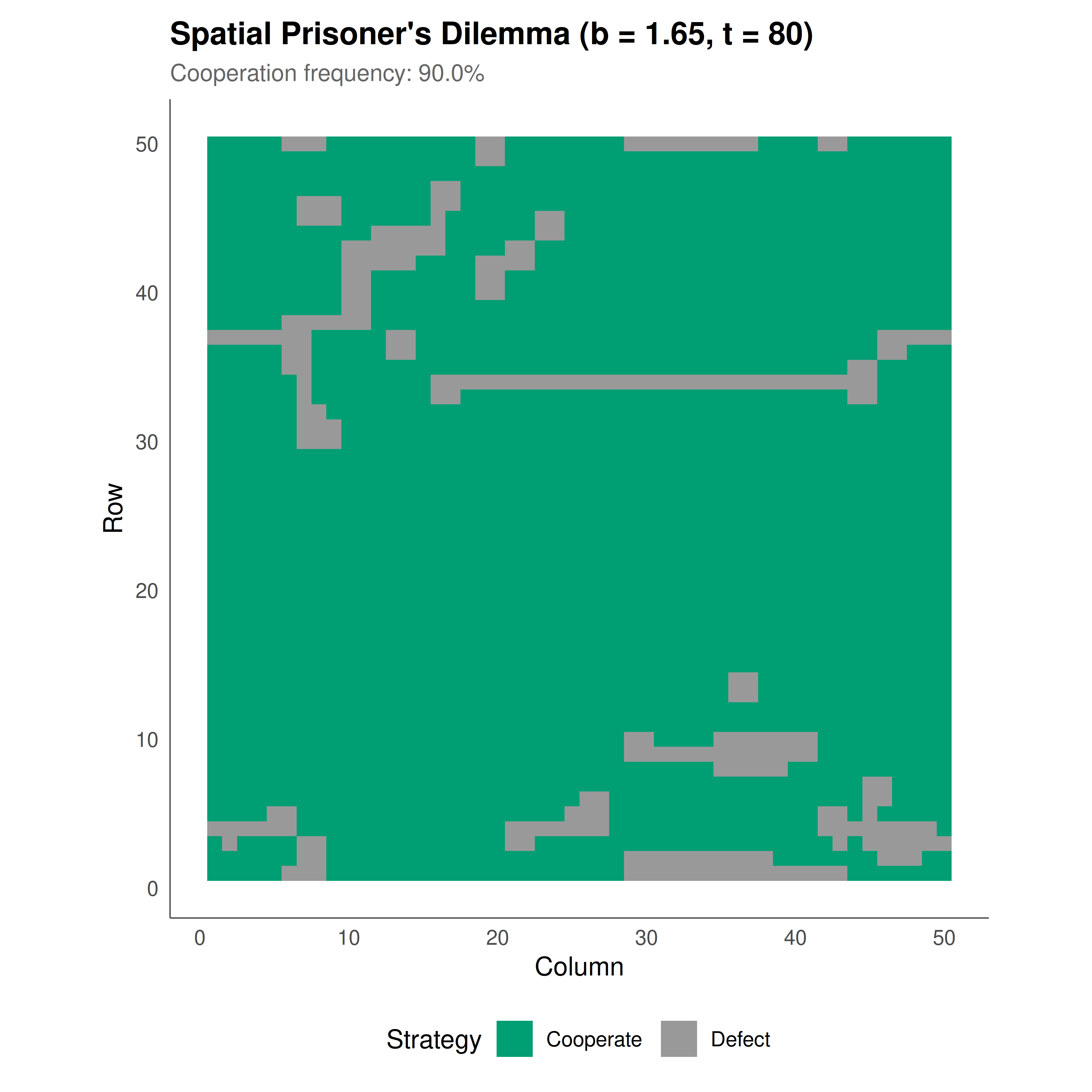
#| fig-cap: "Spatial distribution of cooperators (colored) and defectors (grey) on a 50x50 toroidal lattice after 80 generations of the Nowak-May spatial Prisoner's Dilemma with temptation parameter b = 1.65. Cooperator clusters resist invasion by defectors along their boundaries, creating the characteristic fractal-like patterns of spatial chaos. Rendered using the Okabe-Ito palette."
#| fig-width: 7
#| fig-height: 7
#| dev: [png, pdf]
#| dpi: 300
final_grid <- final_grids[["1.65"]]
grid_df <- expand.grid(x = 1:L, y = 1:L)
grid_df$strategy <- as.vector(final_grid)
grid_df$strategy_label <- ifelse(grid_df$strategy == 1, "Cooperate", "Defect")

ggplot(grid_df, aes(x = x, y = y, fill = strategy_label)) +
  geom_tile() +
  scale_fill_manual(values = c("Cooperate" = okabe_ito[3],
                                "Defect" = okabe_ito[8]),
                    name = "Strategy") +
  labs(title = "Spatial Prisoner's Dilemma (b = 1.65, t = 80)",
       subtitle = sprintf("Cooperation frequency: %.1f%%",
                          mean(final_grid) * 100),
       x = "Column", y = "Row") +
  coord_equal() +
  theme_publication() +
  theme(panel.grid.major = element_blank())
```
## Interactive figure
```{r}
#| label: fig-coop-dynamics-interactive
#| fig-cap: "Interactive time series of cooperation frequency across different temptation parameter values, showing convergence, oscillation, and chaotic dynamics."
p <- ggplot(coop_history, aes(x = step, y = coop_frac, color = b_value,
                               text = paste0("Step: ", step,
                                             "\nCooperation: ",
                                             round(coop_frac * 100, 1), "%",
                                             "\n", b_value))) +
  geom_line(linewidth = 0.7) +
  scale_color_manual(values = okabe_ito[1:3], name = "Temptation") +
  scale_y_continuous(labels = scales::percent_format(),
                     limits = c(0, 1)) +
  labs(title = "Cooperation dynamics on spatial lattice",
       subtitle = "Hover to see exact cooperation levels at each time step",
       x = "Generation", y = "Cooperation frequency") +
  theme_publication()

ggplotly(p, tooltip = "text") |>
  config(displaylogo = FALSE,
         modeBarButtonsToRemove = c("select2d", "lasso2d"))
```
## Interpretation
The spatial Prisoner's Dilemma simulations reveal a striking departure from the well-mixed prediction. In a well-mixed population where every player interacts with every other player, defection is the unique evolutionarily stable strategy regardless of the temptation parameter $b$. Cooperation is completely eliminated. Yet on the spatial lattice, cooperation persists at substantial frequencies across a wide range of $b$ values. This persistence is not the result of sophisticated cognitive abilities, memory of past interactions, or institutional enforcement -- the players are entirely memoryless and follow the simplest possible imitation rule. Spatial structure alone is sufficient to sustain cooperation.
The mechanism behind this result is visible in the static figure showing the lattice state at generation 80. Cooperators form compact clusters where interior cells are entirely surrounded by other cooperators and therefore earn the maximum possible payoff (9, from cooperation with all 8 neighbors plus self-play). Defectors on the boundary of a cooperator cluster exploit adjacent cooperators but also border other defectors, reducing their total payoff. When $b$ is moderate (around 1.5-1.7), the payoff advantage of interior cooperators exceeds the boundary advantage of defectors, and cooperator clusters maintain their integrity. Defectors cannot penetrate the interior because no boundary defector earns more than an interior cooperator. The result is a dynamic equilibrium where the boundary fluctuates but cooperation is never eliminated.
The three time series in the interactive figure illustrate how the temptation parameter $b$ governs the qualitative dynamics. At $b = 1.5$, cooperation stabilizes at a high level because the temptation to defect is insufficient to overcome the cluster defense. At $b = 1.65$, the system enters the chaotic regime identified by Nowak and May: cooperation frequency fluctuates irregularly as clusters form, fragment, and reform in an endless cycle. The spatial patterns at this parameter value exhibit fractal-like structure, with self-similar features at multiple scales. At $b = 1.8$, the temptation is strong enough that defectors erode cooperator clusters more effectively, and cooperation frequency settles at a lower level, though it is typically not zero -- even at high temptation, small cooperator refugia can survive in the lattice geometry.
These results have profound implications for understanding cooperation in biological and social systems. Many real interactions are spatially structured: organisms compete with geographic neighbors, firms compete with local rivals, and social norms spread through contact networks. The Nowak-May model demonstrates that spatial structure is not merely a complication to be abstracted away but a fundamental determinant of strategic outcomes. The transition from stable coexistence through spatial chaos to defector dominance as $b$ increases mirrors phase transitions in statistical physics, connecting game theory to the broader study of complex systems. Extensions of this model to heterogeneous lattices, stochastic update rules, and continuous strategy spaces remain active research topics, and the cellular automaton framework provides an accessible computational laboratory for exploring these questions.
## Extensions & related tutorials
- [Network visualization for games with igraph](../../visualization-and-communication/network-visualization-igraph/) -- Visualize interaction structures on more general network topologies beyond regular lattices.
- [Bayesian inference for game-theoretic parameters](../../statistical-foundations/bayesian-inference-game-parameters/) -- Estimate parameters like $b$ from observed spatial game data.
- [Cointegration analysis of strategic long-run relationships](../../time-series-econometrics/cointegration-strategic-long-run/) -- Test for long-run strategic relationships in time-series data from spatial simulations.
- [Uber surge pricing as a dynamic game](../../real-world-data-applications/uber-surge-pricing-game/) -- Apply dynamic game concepts to spatial platform markets.
- [Literate programming for game theory](../../reproducibility-open-science/literate-programming-game-theory/) -- Document simulation studies for reproducibility.
## References
::: {#refs}
:::