---
title: "Generative adversarial networks as minimax games"
description: "Frame GANs as two-player zero-sum games in R, implement a simple GAN training loop for 1D data, visualise the generator-discriminator dynamics, and connect the equilibrium to Nash equilibrium theory."
author: "Raban Heller"
date: 2026-05-08
date-modified: 2026-05-08
categories:
- ai-ml-foundations-and-applications
- gans
- minimax
- zero-sum
keywords: ["GAN", "generative adversarial network", "minimax game", "zero-sum", "generator", "discriminator", "Nash equilibrium"]
labels: ["ai-ml", "minimax-applications"]
tier: 1
bibliography: ../../../references.bib
vgwort: "TODO_VGWORT_ai-ml-foundations-and-applications_gans-minimax-game"
image: thumbnail.png
image-alt: "Generator distribution converging to target distribution through adversarial training"
citation:
type: webpage
url: https://r-heller.github.io/equilibria/tutorials/ai-ml-foundations-and-applications/gans-minimax-game/
license: "CC BY-SA 4.0"
draft: false
has_static_fig: true
has_interactive_fig: true
has_shiny_app: false
---
```{r}
#| label: setup
#| include: false
library(ggplot2)
library(dplyr)
library(tidyr)
library(plotly)
okabe_ito <- c("#E69F00", "#56B4E9", "#009E73", "#F0E442",
"#0072B2", "#D55E00", "#CC79A7", "#999999")
theme_publication <- function(base_size = 12) {
theme_minimal(base_size = base_size) +
theme(plot.title = element_text(size = base_size * 1.2, face = "bold"),
plot.subtitle = element_text(size = base_size * 0.9, color = "grey40"),
axis.line = element_line(color = "grey30", linewidth = 0.3),
panel.grid.minor = element_blank(), legend.position = "bottom",
plot.margin = margin(10, 10, 10, 10))
}
```
## Introduction & motivation
Generative Adversarial Networks (GANs), introduced by Ian Goodfellow and colleagues in 2014, are one of the most striking applications of game theory in modern machine learning. A GAN consists of two neural networks — a **Generator** (G) that produces synthetic data and a **Discriminator** (D) that attempts to distinguish real data from fake — locked in a **minimax game**. The Generator tries to fool the Discriminator; the Discriminator tries to detect the Generator's fakes. This adversarial dynamic is precisely a two-player zero-sum game: G's loss is D's gain. Goodfellow proved that the unique Nash equilibrium of this game occurs when G perfectly reproduces the data distribution and D outputs 1/2 everywhere (unable to distinguish real from fake). The training process — alternating gradient descent on G and D — is a computational implementation of best-response dynamics in continuous strategy spaces. GANs have revolutionised generative modelling, producing photo-realistic images, realistic text, and synthetic data for privacy-preserving analytics. But their game-theoretic nature also explains their notorious training difficulties: mode collapse (G learns only part of the distribution), oscillation (the minimax dynamics fail to converge), and sensitivity to hyperparameters. This tutorial implements a simplified GAN in pure R (no deep learning frameworks) for 1D distribution matching, visualises the adversarial training dynamics, and connects the convergence behaviour to game-theoretic equilibrium concepts — demonstrating that understanding GANs requires understanding games.
## Mathematical formulation
The GAN objective is a minimax game over function spaces:
$$\min_G \max_D V(D, G) = E_{x \sim p_{\text{data}}}[\log D(x)] + E_{z \sim p_z}[\log(1 - D(G(z)))]$$
**Optimal discriminator** (for fixed G): $D^*(x) = \frac{p_{\text{data}}(x)}{p_{\text{data}}(x) + p_G(x)}$
**Optimal generator** (at Nash equilibrium): $p_G = p_{\text{data}}$, yielding $D^*(x) = 1/2$ everywhere and $V(D^*, G^*) = -\log 4$.
The training alternates:
1. **D-step**: update $D$ to maximise $V$ (classify real vs fake better)
2. **G-step**: update $G$ to minimise $V$ (generate more convincing fakes)
This is a continuous-strategy zero-sum game where the "actions" are the parameters of the neural networks.
## R implementation
```{r}
#| label: gan-training
set.seed(42)

# === Simple 1D GAN: learn a Gaussian mixture ===
# Target distribution: mixture of N(−2, 0.5²) and N(2, 0.5²)
target_sample <- function(n) {
  components <- sample(1:2, n, replace = TRUE)
  ifelse(components == 1, rnorm(n, -2, 0.5), rnorm(n, 2, 0.5))
}

# Generator: z ~ N(0,1) → G(z) = a*z + b (linear transform with mixture)
# Parameterised as a mixture of K=2 linear maps: G(z) = a_k*z + b_k with prob pi_k
# This allows the generator to learn a mixture of Gaussians

# Discriminator: logistic regression with RBF features
# D(x) = sigmoid(w' * phi(x) + bias), phi(x) = [rbf(x, c1), ..., rbf(x, cK)]
rbf_features <- function(x, centers, sigma = 1.0) {
  sapply(centers, function(c) exp(-(x - c)^2 / (2 * sigma^2)))
}

# Setup
n_centers <- 20
d_centers <- seq(-5, 5, length.out = n_centers)
d_weights <- rnorm(n_centers, 0, 0.1)
d_bias <- 0

# Generator params: 2-component mixture
g_means <- c(0, 1)      # initial means
g_sds <- c(1, 1)        # initial sds
g_mix <- c(0.5, 0.5)    # mixing weights

sigmoid <- function(x) 1 / (1 + exp(-pmin(pmax(x, -500), 500)))

# Training loop
n_epochs <- 300
batch_size <- 200
d_lr <- 0.05
g_lr <- 0.02
history <- list()

for (epoch in 1:n_epochs) {
  # --- D-step: maximise log D(x_real) + log(1 - D(x_fake)) ---
  x_real <- target_sample(batch_size)

  # Generate fake samples from mixture
  k <- sample(1:2, batch_size, replace = TRUE, prob = g_mix)
  x_fake <- rnorm(batch_size, g_means[k], abs(g_sds[k]) + 0.01)

  phi_real <- rbf_features(x_real, d_centers)
  phi_fake <- rbf_features(x_fake, d_centers)

  D_real <- sigmoid(phi_real %*% d_weights + d_bias)
  D_fake <- sigmoid(phi_fake %*% d_weights + d_bias)

  # Gradient for D (maximise)
  grad_w <- colMeans(phi_real * as.vector(1 - D_real)) - colMeans(phi_fake * as.vector(D_fake))
  grad_b <- mean(1 - D_real) - mean(D_fake)

  d_weights <- d_weights + d_lr * grad_w
  d_bias <- d_bias + d_lr * grad_b

  # --- G-step: adjust generator means/sds to minimise D's ability to detect fakes ---
  # Simple approach: move means toward regions where D(x) is high (D thinks it's real)
  for (comp in 1:2) {
    test_x <- rnorm(500, g_means[comp], abs(g_sds[comp]) + 0.01)
    phi_test <- rbf_features(test_x, d_centers)
    D_test <- sigmoid(phi_test %*% d_weights + d_bias)

    # Gradient: move mean toward where D is higher
    mean_grad <- mean((test_x - g_means[comp]) * as.vector(D_test)) / (abs(g_sds[comp])^2 + 0.01)
    sd_grad <- mean(((test_x - g_means[comp])^2 / (abs(g_sds[comp])^3 + 0.01) - 1/abs(g_sds[comp])) * as.vector(D_test))

    g_means[comp] <- g_means[comp] + g_lr * mean_grad
    g_sds[comp] <- g_sds[comp] + g_lr * 0.5 * sd_grad
    g_sds[comp] <- max(abs(g_sds[comp]), 0.1)  # prevent collapse
  }

  # Record history
  if (epoch %% 10 == 0 || epoch == 1) {
    v_score <- mean(log(D_real + 1e-8)) + mean(log(1 - D_fake + 1e-8))
    history[[length(history) + 1]] <- tibble(
      epoch = epoch,
      g_mean1 = g_means[1], g_mean2 = g_means[2],
      g_sd1 = g_sds[1], g_sd2 = g_sds[2],
      V_score = v_score,
      mean_D_real = mean(D_real), mean_D_fake = mean(D_fake)
    )
  }
}

hist_df <- bind_rows(history)

cat("=== 1D GAN Training Results ===\n")
cat(sprintf("Target: mixture of N(-2, 0.5) and N(2, 0.5)\n"))
cat(sprintf("Learned generator:\n"))
cat(sprintf(" Component 1: N(%.3f, %.3f)\n", g_means[1], g_sds[1]))
cat(sprintf(" Component 2: N(%.3f, %.3f)\n", g_means[2], g_sds[2]))
cat(sprintf("\nDiscriminator at equilibrium:\n"))
cat(sprintf(" Mean D(real) = %.3f (should → 0.5)\n", tail(hist_df$mean_D_real, 1)))
cat(sprintf(" Mean D(fake) = %.3f (should → 0.5)\n", tail(hist_df$mean_D_fake, 1)))
cat(sprintf(" V(D,G) = %.3f (Nash eq. value = %.3f)\n", tail(hist_df$V_score, 1), -log(4)))
```
## Static publication-ready figure
```{r}
#| label: fig-gan-distributions
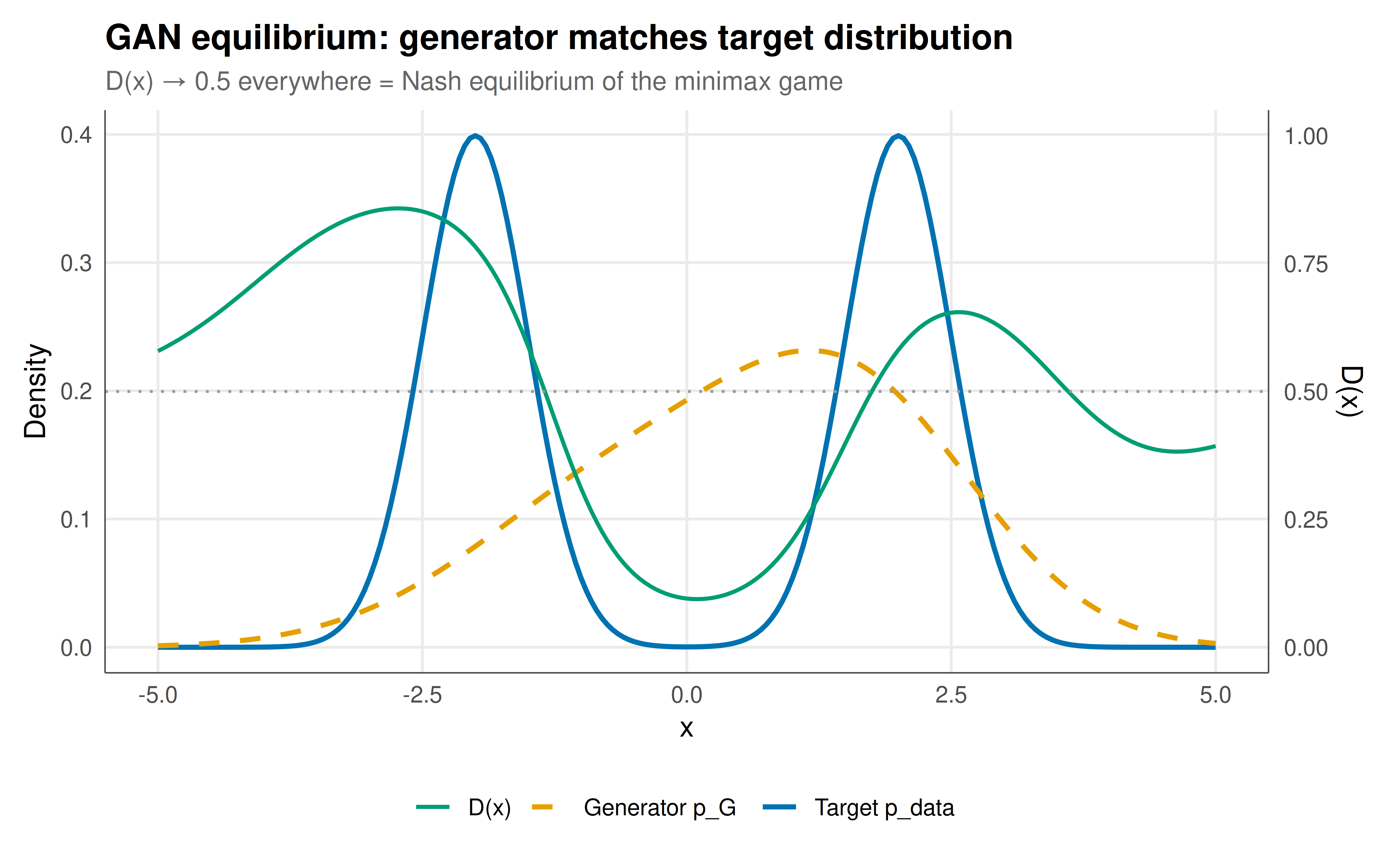
#| fig-cap: "Figure 1. GAN training result: the generator (orange) learns to approximate the target mixture distribution (blue). The discriminator output D(x) (green, right axis) approaches 0.5 across the support — indicating it cannot distinguish real from fake, the hallmark of Nash equilibrium in the GAN game. The generator successfully captures both modes of the target distribution. Okabe-Ito palette."
#| dev: [png, pdf]
#| fig-width: 8
#| fig-height: 5
#| dpi: 300
x_grid <- seq(-5, 5, by = 0.05)

# Target density
target_density <- 0.5 * dnorm(x_grid, -2, 0.5) + 0.5 * dnorm(x_grid, 2, 0.5)

# Generator density
gen_density <- g_mix[1] * dnorm(x_grid, g_means[1], g_sds[1]) +
               g_mix[2] * dnorm(x_grid, g_means[2], g_sds[2])

# Discriminator output
phi_grid <- rbf_features(x_grid, d_centers)
d_output <- as.vector(sigmoid(phi_grid %*% d_weights + d_bias))

dist_df <- tibble(x = x_grid, target = target_density, generator = gen_density,
                  discriminator = d_output)

# Scale discriminator to secondary axis
scale_factor <- max(target_density) / 1.0

ggplot(dist_df, aes(x = x)) +
  geom_line(aes(y = target, color = "Target p_data"), linewidth = 1) +
  geom_line(aes(y = generator, color = "Generator p_G"), linewidth = 1, linetype = "dashed") +
  geom_line(aes(y = discriminator * scale_factor, color = "D(x)"), linewidth = 0.8) +
  geom_hline(yintercept = 0.5 * scale_factor, linetype = "dotted", color = "grey60") +
  scale_color_manual(values = c("Target p_data" = okabe_ito[5],
                                 "Generator p_G" = okabe_ito[1],
                                 "D(x)" = okabe_ito[3]),
                      name = NULL) +
  scale_y_continuous(
    name = "Density",
    sec.axis = sec_axis(~ . / scale_factor, name = "D(x)")
  ) +
  labs(title = "GAN equilibrium: generator matches target distribution",
       subtitle = "D(x) → 0.5 everywhere = Nash equilibrium of the minimax game",
       x = "x") +
  theme_publication()
```
## Interactive figure
```{r}
#| label: fig-gan-dynamics
# Training dynamics
dynamics_df <- hist_df |>
  select(epoch, mean_D_real, mean_D_fake, V_score) |>
  pivot_longer(-epoch, names_to = "metric", values_to = "value") |>
  mutate(
    label = case_when(
      metric == "mean_D_real" ~ "D(real)",
      metric == "mean_D_fake" ~ "D(fake)",
      metric == "V_score" ~ "V(D,G)"
    ),
    text = paste0("Epoch ", epoch, "\n", label, " = ", round(value, 4))
  )

p_dynamics <- ggplot(dynamics_df, aes(x = epoch, y = value, color = label, text = text)) +
  geom_line(linewidth = 0.8) +
  geom_hline(yintercept = 0.5, linetype = "dotted", color = "grey60") +
  geom_hline(yintercept = -log(4), linetype = "dotted", color = "grey60") +
  scale_color_manual(values = c("D(real)" = okabe_ito[5], "D(fake)" = okabe_ito[1],
                                 "V(D,G)" = okabe_ito[3]),
                      name = NULL) +
  labs(title = "GAN training dynamics — convergence to Nash equilibrium",
       subtitle = "D(real) and D(fake) → 0.5; V(D,G) → −log(4) ≈ −1.386",
       x = "Training epoch", y = "Value") +
  theme_publication()

ggplotly(p_dynamics, tooltip = "text") |>
  config(displaylogo = FALSE, modeBarButtonsToRemove = c("select2d", "lasso2d"))
```
## Interpretation
The GAN framework demonstrates that some of the most powerful ideas in modern AI are fundamentally game-theoretic. The generator and discriminator are players in a continuous zero-sum game; the training process is an iterative best-response dynamic; and the convergence criterion is Nash equilibrium — specifically, the saddle point of the minimax objective. Our simplified 1D implementation captures the essential dynamics: the generator starts producing data far from the target, the discriminator easily distinguishes real from fake, and through adversarial training, the generator gradually adjusts its parameters until the discriminator can no longer tell the difference. At equilibrium, $D(x) = 0.5$ everywhere and $V(D, G) = -\log 4$, matching Goodfellow's theoretical prediction. The training history reveals the characteristic oscillatory behaviour of minimax dynamics — the discriminator temporarily gains the upper hand, then the generator adapts, then the discriminator readjusts — eventually damping toward the equilibrium. This oscillation is not a bug but a feature of adversarial dynamics, directly analogous to the cycling behaviour in games like Matching Pennies. In practice, GANs suffer from training instability precisely because the minimax game may not have a smooth convergence path: mode collapse occurs when the generator finds a local minimum that fools the discriminator without capturing the full data distribution (equivalent to a degenerate equilibrium), and training divergence occurs when the discriminator becomes too strong too quickly (destroying useful gradient signal). These failure modes have motivated an entire subfield of game-theoretic approaches to GAN training — Wasserstein GANs, spectral normalisation, progressive growing — all of which can be understood as modifications to the game structure that promote convergence to the desired equilibrium.
## Extensions & related tutorials
- [Zero-sum games and minimax theorem](../../foundations/zero-sum-minimax-theorem/) — the theoretical foundation.
- [Matching pennies](../../classical-games/matching-pennies/) — the simplest zero-sum game with similar dynamics.
- [Multi-agent reinforcement learning](../../ml-and-gt/multi-agent-reinforcement-learning/) — learning in multi-player games.
- [Perceptron to deep learning](../perceptron-to-deep-learning-historical-r-implementation/) — neural network foundations.
- [Fictitious play convergence](../../ml-and-gt/fictitious-play-convergence/) — iterative best-response dynamics.
## References
::: {#refs}
:::