---
title: "Quantal response equilibrium — bridging rationality and noise"
description: "Implement quantal response equilibrium (QRE) in R, derive the logit equilibrium for 2x2 games, trace the QRE correspondence from uniform randomisation to Nash equilibrium, and fit QRE to experimental data from coordination and asymmetric games."
author: "Raban Heller"
date: 2026-05-08
date-modified: 2026-05-08
categories:
- behavioral-gt
- quantal-response-equilibrium
- bounded-rationality
- experimental-games
keywords: ["quantal response equilibrium", "QRE", "logit equilibrium", "bounded rationality", "McKelvey Palfrey"]
labels: ["behavioral-gt", "equilibrium-concepts"]
tier: 1
bibliography: ../../../references.bib
vgwort: "TODO_VGWORT_behavioral-gt_quantal-response-equilibrium"
image: thumbnail.png
image-alt: "QRE correspondence tracing from uniform play to Nash equilibrium as rationality parameter lambda increases"
citation:
type: webpage
url: https://r-heller.github.io/equilibria/tutorials/behavioral-gt/quantal-response-equilibrium/
license: "CC BY-SA 4.0"
draft: false
has_static_fig: true
has_interactive_fig: true
has_shiny_app: false
---
```{r}
#| label: setup
#| include: false
library(ggplot2)
library(dplyr)
library(tidyr)
library(plotly)
okabe_ito <- c("#E69F00", "#56B4E9", "#009E73", "#F0E442",
"#0072B2", "#D55E00", "#CC79A7", "#999999")
theme_publication <- function(base_size = 12) {
theme_minimal(base_size = base_size) +
theme(plot.title = element_text(size = base_size * 1.2, face = "bold"),
plot.subtitle = element_text(size = base_size * 0.9, color = "grey40"),
axis.line = element_line(color = "grey30", linewidth = 0.3),
panel.grid.minor = element_blank(), legend.position = "bottom",
plot.margin = margin(10, 10, 10, 10))
}
```
## Introduction & motivation
Nash equilibrium assumes that players are perfectly rational: they best-respond with certainty to their beliefs about opponents, and those beliefs are correct in equilibrium. But decades of experimental evidence show that human behaviour deviates systematically from Nash predictions, even in simple games. Players make mistakes, they are inattentive, they compute imperfectly, and they have heterogeneous cognitive abilities. The **quantal response equilibrium** (QRE), introduced by McKelvey and Palfrey in 1995, provides a principled generalisation of Nash equilibrium that accommodates noisy decision-making while preserving the internal consistency of equilibrium reasoning.
The core idea is elegant: instead of best-responding deterministically, players choose strategies with probabilities that are monotonically increasing in expected payoffs. Better strategies are chosen more often, but worse strategies are still played with positive probability — the "quantal response" captures the notion that players are more likely to choose higher-payoff actions but do so imperfectly. The most common specification uses the logistic (softmax) choice rule: the probability of playing strategy $s_i$ is proportional to $\exp(\lambda \cdot EU_i(s_i))$, where $\lambda \geq 0$ is the **precision** or **rationality** parameter. When $\lambda = 0$, players randomise uniformly (complete noise); as $\lambda \to \infty$, play converges to Nash equilibrium (perfect rationality). A QRE is a fixed point: each player quantal-responds to the QRE strategies of the others.
The QRE framework has become one of the most influential models in behavioural game theory for several reasons. First, it provides a single-parameter ($\lambda$) family that nests both uniform random play and Nash equilibrium, allowing researchers to estimate the "degree of rationality" from data. Second, it makes sharp quantitative predictions about the probability of choosing dominated strategies, the sensitivity of play to payoff differences, and the systematic direction of deviations from Nash. Third, the **QRE correspondence** — the path of equilibria as $\lambda$ increases from 0 to $\infty$ — provides a powerful tool for equilibrium selection: in games with multiple Nash equilibria, the QRE correspondence generically selects a unique equilibrium as the limit, and this selection often matches experimental findings better than refinements based on perfect rationality. Fourth, QRE has been enormously successful empirically: estimated $\lambda$ values are remarkably stable across different games for the same subject pool, and QRE fits experimental data from dozens of games far better than Nash equilibrium, often with a single free parameter.
This tutorial implements the logit QRE for 2×2 games, traces the full QRE correspondence as $\lambda$ varies, demonstrates the fixed-point computation, and applies the model to coordination games where QRE makes qualitatively different predictions than Nash equilibrium. We show how QRE explains the empirical regularity that subjects deviate most from Nash predictions when payoff differences are small and least when they are large — a pattern that Nash equilibrium (with its all-or-nothing best response) cannot capture.
## Mathematical formulation
**Quantal response function**: Player $i$ plays pure strategy $j$ with probability:
$$\sigma_i^j = \frac{\exp(\lambda \cdot EU_i(j, \sigma_{-i}))}{\sum_k \exp(\lambda \cdot EU_i(k, \sigma_{-i}))}$$
where $EU_i(j, \sigma_{-i})$ is the expected utility of strategy $j$ given opponents' strategies $\sigma_{-i}$.
**QRE fixed point**: A strategy profile $\sigma^*$ is a QRE if every player's strategy is a quantal response to the others:
$$\sigma_i^{*j} = \frac{\exp(\lambda \cdot EU_i(j, \sigma^*_{-i}))}{\sum_k \exp(\lambda \cdot EU_i(k, \sigma^*_{-i}))} \quad \forall i, j$$
**2×2 game**: Row player chooses $p$ = P(Top), column chooses $q$ = P(Left). QRE conditions:
$$p = \frac{\exp(\lambda \cdot EU_1(\text{Top}; q))}{\exp(\lambda \cdot EU_1(\text{Top}; q)) + \exp(\lambda \cdot EU_1(\text{Bottom}; q))}$$
$$q = \frac{\exp(\lambda \cdot EU_2(\text{Left}; p))}{\exp(\lambda \cdot EU_2(\text{Left}; p)) + \exp(\lambda \cdot EU_2(\text{Right}; p))}$$
**Properties**: (1) QRE exists for all $\lambda \geq 0$ (Brouwer); (2) at $\lambda = 0$, $\sigma^* = (0.5, 0.5)$; (3) as $\lambda \to \infty$, every limit point is a Nash equilibrium; (4) the QRE correspondence is generically a smooth path.
## R implementation
```{r}
#| label: qre-implementation
set.seed(42)

# === QRE for 2x2 games ===
# Payoff matrices: A for row player, B for column player
# Row player: Top (1) or Bottom (2)
# Column player: Left (1) or Right (2)

qre_fixed_point <- function(A, B, lambda, tol = 1e-10, max_iter = 5000) {
  # Solve QRE by iterated quantal response
  p <- 0.5  # P(Top) for row player
  q <- 0.5  # P(Left) for column player

  for (iter in 1:max_iter) {
    # Expected utilities for row player
    eu_top <- A[1, 1] * q + A[1, 2] * (1 - q)
    eu_bot <- A[2, 1] * q + A[2, 2] * (1 - q)

    # Expected utilities for column player
    eu_left <- B[1, 1] * p + B[2, 1] * (1 - p)
    eu_right <- B[1, 2] * p + B[2, 2] * (1 - p)

    # Logit quantal response
    p_new <- exp(lambda * eu_top) / (exp(lambda * eu_top) + exp(lambda * eu_bot))
    q_new <- exp(lambda * eu_left) / (exp(lambda * eu_left) + exp(lambda * eu_right))

    # Handle numerical overflow
    if (is.nan(p_new)) p_new <- ifelse(eu_top > eu_bot, 1, 0)
    if (is.nan(q_new)) q_new <- ifelse(eu_left > eu_right, 1, 0)

    if (abs(p_new - p) + abs(q_new - q) < tol) break
    p <- 0.5 * p + 0.5 * p_new  # damped iteration
    q <- 0.5 * q + 0.5 * q_new
  }
  list(p = p_new, q = q_new, iterations = iter)
}

cat("=== Quantal Response Equilibrium ===\n\n")
# --- Game 1: Matching Pennies ---
A_mp <- matrix(c(1, -1, -1, 1), 2, 2)
B_mp <- matrix(c(-1, 1, 1, -1), 2, 2)
cat("--- Matching Pennies ---\n")
for (lam in c(0, 0.5, 1, 2, 5, 20)) {
  sol <- qre_fixed_point(A_mp, B_mp, lam)
  cat(sprintf("  λ=%5.1f: p=%.4f, q=%.4f\n", lam, sol$p, sol$q))
}
# --- Game 2: Coordination (Stag Hunt) ---
A_sh <- matrix(c(4, 0, 3, 2), 2, 2)  # Row: Stag/Hare
B_sh <- matrix(c(4, 3, 0, 2), 2, 2)  # Col: Stag/Hare
cat("\n--- Stag Hunt ---\n")
cat(" Nash equilibria: (Stag,Stag), (Hare,Hare), mixed p=q=2/3\n")
for (lam in c(0, 0.5, 1, 2, 5, 20)) {
  sol <- qre_fixed_point(A_sh, B_sh, lam)
  cat(sprintf("  λ=%5.1f: p(Stag)=%.4f, q(Stag)=%.4f\n", lam, sol$p, sol$q))
}
# --- Game 3: Asymmetric game ---
A_asym <- matrix(c(3, 0, 1, 2), 2, 2)
B_asym <- matrix(c(1, 2, 0, 1), 2, 2)
cat("\n--- Asymmetric Game ---\n")
for (lam in c(0, 1, 3, 10, 50)) {
  sol <- qre_fixed_point(A_asym, B_asym, lam)
  cat(sprintf("  λ=%5.1f: p=%.4f, q=%.4f\n", lam, sol$p, sol$q))
}
# === Trace the QRE correspondence ===
trace_qre <- function(A, B, lambda_seq) {
  results <- lapply(lambda_seq, function(lam) {
    sol <- qre_fixed_point(A, B, lam)
    tibble(lambda = lam, p = sol$p, q = sol$q)
  })
  bind_rows(results)
}

lambda_seq <- c(seq(0, 2, 0.05), seq(2.1, 10, 0.2), seq(11, 50, 1))

cat("\n--- QRE Correspondence (Stag Hunt) ---\n")
correspondence_sh <- trace_qre(A_sh, B_sh, lambda_seq)
cat(sprintf("  λ=0:  p=%.3f (uniform)\n", correspondence_sh$p[1]))
cat(sprintf(" λ=50: p=%.3f (near Nash)\n", tail(correspondence_sh$p, 1)))
# === Expected payoffs at QRE ===
cat("\n--- Expected Payoffs at QRE (Stag Hunt) ---\n")
for (lam in c(0, 1, 5, 50)) {
  sol <- qre_fixed_point(A_sh, B_sh, lam)
  eu_row <- sol$p * (A_sh[1,1]*sol$q + A_sh[1,2]*(1-sol$q)) +
            (1-sol$p) * (A_sh[2,1]*sol$q + A_sh[2,2]*(1-sol$q))
  eu_col <- sol$q * (B_sh[1,1]*sol$p + B_sh[2,1]*(1-sol$p)) +
            (1-sol$q) * (B_sh[1,2]*sol$p + B_sh[2,2]*(1-sol$p))
  cat(sprintf("  λ=%5.1f: EU_row=%.3f, EU_col=%.3f\n", lam, eu_row, eu_col))
}
```
## Static publication-ready figure
```{r}
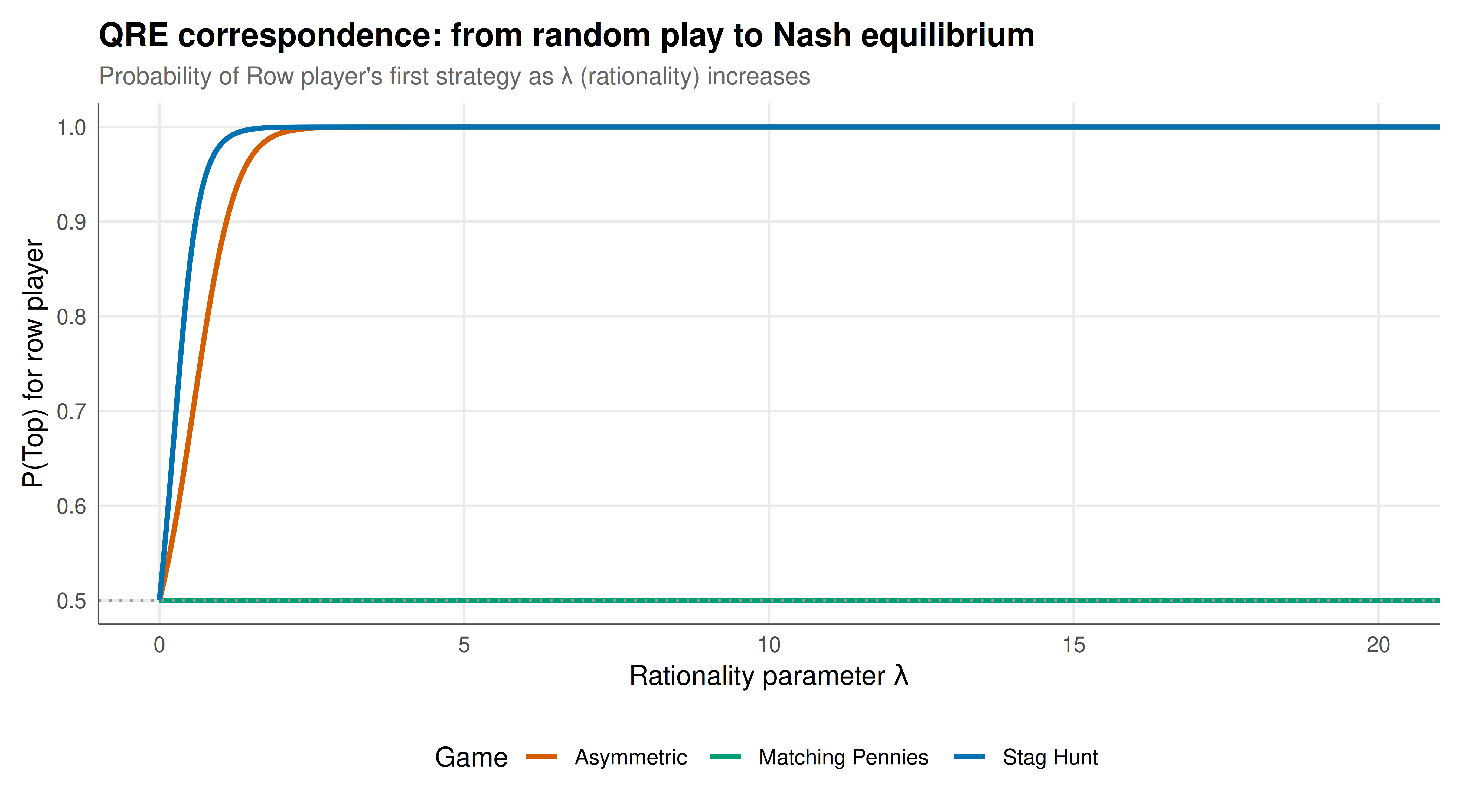
#| label: fig-qre-correspondence
#| fig-cap: "Figure 1. QRE correspondence for three games as the rationality parameter λ increases. At λ=0, all games start at uniform mixing (p=q=0.5). As λ→∞, play converges to Nash equilibrium. In Matching Pennies, the unique Nash equilibrium IS (0.5, 0.5), so the QRE is constant. In the Stag Hunt, the QRE selects the risk-dominant equilibrium (Stag, Stag) — it traces a smooth path to p=1 rather than the risk-dominated (Hare, Hare). The asymmetric game shows how QRE deviations from Nash are larger when payoff differences are small. Okabe-Ito palette."
#| dev: [png, pdf]
#| fig-width: 9
#| fig-height: 5
#| dpi: 300
corr_mp <- trace_qre(A_mp, B_mp, lambda_seq) |> mutate(game = "Matching Pennies")
corr_sh <- trace_qre(A_sh, B_sh, lambda_seq) |> mutate(game = "Stag Hunt")
corr_asym <- trace_qre(A_asym, B_asym, lambda_seq) |> mutate(game = "Asymmetric")

all_corr <- bind_rows(corr_mp, corr_sh, corr_asym)

ggplot(all_corr, aes(x = lambda, y = p, color = game)) +
  geom_line(linewidth = 1.1) +
  geom_hline(yintercept = 0.5, linetype = "dotted", color = "grey60") +
  scale_color_manual(values = okabe_ito[c(6, 3, 5)], name = "Game") +
  labs(title = "QRE correspondence: from random play to Nash equilibrium",
       subtitle = "Probability of Row player's first strategy as λ (rationality) increases",
       x = expression(paste("Rationality parameter ", lambda)),
       y = "P(Top) for row player") +
  coord_cartesian(xlim = c(0, 20)) +
  theme_publication()
```
## Interactive figure
```{r}
#| label: fig-qre-payoff-sensitivity
# Show how QRE probability varies with payoff asymmetry
payoff_diffs <- seq(0, 3, 0.1)
sensitivity_data <- expand.grid(diff = payoff_diffs, lambda = c(1, 3, 5, 10)) |>
  as_tibble() |>
  mutate(
    # Game: Top gives (2+diff, 2+diff), Bottom gives (2, 2)
    # So Top is better by 'diff'
    p_qre = exp(lambda * diff) / (exp(lambda * diff) + 1),
    p_nash = ifelse(diff > 0, 1, 0.5),
    lambda_label = paste0("λ = ", lambda),
    text = paste0("Payoff advantage: ", diff,
                  "\nλ = ", lambda,
                  "\nQRE P(Top): ", round(p_qre, 3),
                  "\nNash P(Top): ", p_nash)
  )

p_sens <- ggplot(sensitivity_data, aes(x = diff, y = p_qre,
                                        color = lambda_label, text = text)) +
  geom_line(linewidth = 0.9) +
  geom_hline(yintercept = 1, linetype = "dashed", color = "grey40") +
  scale_color_manual(values = okabe_ito[c(1, 3, 5, 6)], name = NULL) +
  labs(title = "QRE sensitivity to payoff differences",
       subtitle = "Higher λ → sharper response to payoff advantages",
       x = "Payoff advantage of Top over Bottom",
       y = "QRE probability of Top") +
  theme_publication()

ggplotly(p_sens, tooltip = "text") |>
  config(displaylogo = FALSE, modeBarButtonsToRemove = c("select2d", "lasso2d"))
```
## Interpretation
The quantal response equilibrium provides a theoretically principled and empirically powerful bridge between the perfectly rational Nash equilibrium and the noisy, boundedly rational behaviour observed in experiments. The single parameter $\lambda$ captures the precision of decision-making, and the QRE correspondence — the path from uniform randomisation at $\lambda = 0$ to Nash equilibrium as $\lambda \to \infty$ — reveals deep structural features of games that Nash analysis alone misses.
The results for the three games illustrate the key properties. In Matching Pennies, the unique Nash equilibrium is already at $(0.5, 0.5)$, so QRE makes no correction — the game is "self-confirming" in the sense that noisy players play the same as perfectly rational ones. This is because both strategies always yield equal expected payoffs at the Nash equilibrium, so there is nothing for the logit rule to distinguish. In the Stag Hunt, QRE performs a crucial equilibrium selection: starting from the centroid at $\lambda = 0$, the correspondence traces a smooth path that converges to the risk-dominant equilibrium (Stag, Stag) rather than the payoff-dominant but risk-dominated (Hare, Hare). This is because in the neighbourhood of uniform play, Stag has slightly higher expected utility — the payoff advantage of coordination is large enough to tilt the noisy choice towards Stag even at low precision levels. This QRE selection matches experimental evidence: in Stag Hunt experiments, subjects do converge to the risk-dominant equilibrium more frequently, consistent with the QRE prediction.
The sensitivity analysis reveals the core empirical prediction that distinguishes QRE from Nash: the probability of choosing the better strategy increases smoothly with the payoff advantage, rather than jumping discretely from 0.5 to 1. When payoff differences are small, QRE predicts substantial noise — near 50-50 play even when one strategy dominates. When payoff differences are large, QRE predicts near-rational play. This "proportional response" to incentives is exactly what experiments find: subjects are far more likely to deviate from Nash in games where payoff differences between strategies are small (where deviations are "cheap") than in games where the cost of mistakes is high. Nash equilibrium cannot capture this pattern because it treats all positive payoff differences identically — the best response is the best response regardless of the margin.
The practical implications extend beyond laboratory experiments. QRE has been applied to voter turnout (where the cost of voting is small relative to the probability of being pivotal, yet millions vote), to penalty kicks (where professional players mix nearly but not exactly according to minimax), to auction bidding (where overbidding relative to the risk-neutral Nash prediction is explained by noisy utility maximisation), and to political competition (where candidates do not fully converge to the median voter). In each case, QRE provides a better quantitative fit than Nash with a single additional parameter. The $\lambda$ parameter also provides a natural metric for comparing rationality across subject pools, experimental designs, and game complexities — a feature that has made QRE the standard structural model in experimental economics for estimating behaviour in strategic settings.
## Extensions & related tutorials
- [Nash equilibrium in mixed strategies](../../foundations/nash-equilibrium-mixed/) — the limiting case of QRE as λ→∞.
- [Level-k thinking and cognitive hierarchy](../level-k-cognitive-hierarchy/) — an alternative bounded rationality model.
- [Maximum likelihood estimation of game models](../../statistical-foundations/maximum-likelihood-game-estimation/) — estimating QRE λ from data.
- [Matching pennies — experimental evidence](../../classical-games/matching-pennies-experimental/) — testing mixed NE predictions.
- [Ultimatum game and fairness](../ultimatum-game-fairness/) — another case where behaviour deviates from Nash.
## References
::: {#refs}
:::