---
title: "Maximum Likelihood Estimation of Game-Theoretic Models"
description: "Estimate the quantal response equilibrium (QRE) rationality parameter from experimental choice data using maximum likelihood, visualize the log-likelihood surface, and compare QRE with Nash equilibrium predictions."
author: "Raban Heller"
date: 2026-05-08
date-modified: 2026-05-08
categories:
- statistical-foundations
- maximum-likelihood
- quantal-response-equilibrium
keywords: ["maximum likelihood estimation", "quantal response equilibrium", "QRE", "logit equilibrium", "experimental games"]
labels: ["statistics", "estimation"]
tier: 1
bibliography: ../../../references.bib
vgwort: "TODO_VGWORT_statistical-foundations_maximum-likelihood-game-estimation"
image: thumbnail.png
image-alt: "Log-likelihood surface for QRE lambda parameter estimation with maximum likelihood point and confidence interval marked"
citation:
type: webpage
url: https://r-heller.github.io/equilibria/tutorials/statistical-foundations/maximum-likelihood-game-estimation/
license: "CC BY-SA 4.0"
draft: false
has_static_fig: true
has_interactive_fig: true
has_shiny_app: false
---
```{r}
#| label: setup
#| include: false
library(ggplot2)
library(dplyr)
library(tidyr)
library(plotly)
okabe_ito <- c("#E69F00", "#56B4E9", "#009E73", "#F0E442",
"#0072B2", "#D55E00", "#CC79A7", "#999999")
theme_publication <- function(base_size = 12) {
theme_minimal(base_size = base_size) +
theme(plot.title = element_text(size = base_size * 1.2, face = "bold"),
plot.subtitle = element_text(size = base_size * 0.9, color = "grey40"),
axis.line = element_line(color = "grey30", linewidth = 0.3),
panel.grid.minor = element_blank(), legend.position = "bottom",
plot.margin = margin(10, 10, 10, 10))
}
```
## Introduction & motivation
The Nash equilibrium concept, foundational to modern game theory since the work of @nash_1950 and @nash_1951, assumes that players are perfectly rational and hold correct beliefs about other players' strategies. While this assumption yields sharp predictions and elegant theoretical results, a large body of experimental evidence has demonstrated that human behavior in strategic settings deviates systematically from Nash predictions. Players make errors, exhibit bounded rationality, and respond to payoff differences in a graded rather than all-or-nothing fashion. The quantal response equilibrium (QRE), introduced by Richard McKelvey and Thomas Palfrey in 1995, provides a principled generalization of Nash equilibrium that accommodates noisy decision-making while preserving the equilibrium requirement of mutual consistency. In a QRE, each player chooses actions with probabilities that are monotonically increasing in expected payoffs --- better actions are chosen more frequently, but even suboptimal actions receive positive probability. The degree of noise in decision-making is governed by a rationality parameter $\lambda$, which ranges from zero (completely random behavior) to infinity (perfect best-response, i.e., Nash equilibrium).
The statistical estimation of the QRE parameter $\lambda$ from experimental data is a central task in behavioral game theory. Given a dataset of observed choices from a strategic game, we want to find the value of $\lambda$ that makes the observed choices most likely under the QRE model. This is a maximum likelihood estimation (MLE) problem: we specify the probability of each observed choice as a function of $\lambda$ (through the QRE choice probabilities), form the likelihood function as the product of these probabilities across all observations, and find the value of $\lambda$ that maximizes this function. The log-likelihood function, being a concave transformation of the likelihood, is typically well-behaved and can be maximized numerically using standard optimization routines such as R's `optim()` function.
This tutorial develops the complete MLE pipeline for QRE estimation from the ground up. We begin by specifying a concrete game --- a symmetric 2x2 game with a unique mixed-strategy Nash equilibrium --- and deriving the QRE choice probabilities as a function of $\lambda$. We then simulate experimental data from a known QRE with a specified $\lambda$ value, ensuring that we have a ground truth against which to validate our estimator. The core of the tutorial constructs the log-likelihood function, applies numerical optimization to find the MLE $\hat{\lambda}$, and computes confidence intervals using both the Hessian-based (observed Fisher information) approach and profile likelihood. We visualize the log-likelihood surface to provide geometric intuition for the estimation, showing how the curvature of the log-likelihood at the maximum determines the precision of the estimate.
The comparison between the QRE model and the Nash equilibrium prediction ($\lambda \to \infty$) is a recurring theme. As $\lambda$ increases, the QRE choice probabilities converge to the Nash equilibrium mixed strategy (or, in games with a unique pure-strategy equilibrium, to deterministic play of that equilibrium). The estimated $\lambda$ thus provides a quantitative measure of how far observed behavior deviates from Nash predictions. Low values of $\hat{\lambda}$ indicate substantial noise or bounded rationality, while high values indicate near-rational play. This interpretation makes QRE estimation a useful diagnostic tool for assessing the descriptive adequacy of Nash equilibrium in any given experimental setting.
Maximum likelihood estimation of game-theoretic models raises several methodological issues that go beyond standard MLE in non-strategic settings. The QRE choice probabilities are implicitly defined by a fixed-point equation --- each player's choice probabilities must be optimal given the other player's (probabilistic) strategy, which in turn depends on the first player's strategy. This means that evaluating the likelihood for a given $\lambda$ requires solving the QRE fixed-point problem, which is itself a nonlinear equation. For 2x2 games, this fixed-point problem can often be solved analytically or reduces to a one-dimensional root-finding problem, but for larger games, it requires iterative numerical methods. This tutorial focuses on the 2x2 case to keep the exposition transparent, but the principles extend directly to larger games.
The techniques developed here --- constructing likelihood functions, performing numerical optimization with `optim()`, computing standard errors from the Hessian, and visualizing likelihood surfaces --- are broadly applicable across computational social science. They appear in the estimation of discrete choice models, structural econometric models, statistical models of network formation, and many other contexts where game-theoretic considerations shape the data-generating process.
## Mathematical formulation
Consider a symmetric $2 \times 2$ game with payoff matrix:
$$
\begin{pmatrix}
(a,\,a) & (b,\,c) \\
(c,\,b) & (d,\,d)
\end{pmatrix}
$$
We use a **Hawk-Dove** parametrization: $a = 0$ (both Hawk), $b = 1$ (Dove vs Hawk), $c = 3$ (Hawk vs Dove), $d = 2$ (both Dove).
Let $p$ denote the probability that a player chooses action 1 (Hawk). The expected payoffs are:
$$
\pi_H(p) = a \cdot p + c \cdot (1-p) = 3 - 3p
$$
$$
\pi_D(p) = b \cdot p + d \cdot (1-p) = 2 - p
$$
**Logit QRE.** In a symmetric logit QRE, the choice probability satisfies the fixed-point condition:
$$
p = \frac{\exp(\lambda \cdot \pi_H(p))}{\exp(\lambda \cdot \pi_H(p)) + \exp(\lambda \cdot \pi_D(p))} = \frac{1}{1 + \exp\bigl(-\lambda [\pi_H(p) - \pi_D(p)]\bigr)}
$$
The payoff difference is:
$$
\Delta\pi(p) = \pi_H(p) - \pi_D(p) = (3 - 3p) - (2 - p) = 1 - 2p
$$
So the fixed-point equation becomes:
$$
p = \frac{1}{1 + \exp(-\lambda(1 - 2p))}
$$
**Nash equilibrium** ($\lambda \to \infty$): $\Delta\pi(p) = 0 \Rightarrow p^* = 1/2$.
**Log-likelihood.** Given $N$ independent observations where $k$ players chose Hawk:
$$
\ell(\lambda) = k \log p(\lambda) + (N - k) \log(1 - p(\lambda))
$$
where $p(\lambda)$ solves the QRE fixed-point equation for parameter $\lambda$.
**Fisher information** and **asymptotic variance**:
$$
\text{Var}(\hat{\lambda}) \approx \left[-\frac{d^2 \ell}{d\lambda^2}\bigg|_{\lambda = \hat{\lambda}}\right]^{-1}
$$
## R implementation
```{r}
#| label: qre-mle
#| code-fold: false
set.seed(2024)

# --- Game parameters (Hawk-Dove) ---
a_pay <- 0; b_pay <- 1; c_pay <- 3; d_pay <- 2

cat("Payoff matrix (Hawk-Dove):\n")
cat(" Hawk Dove\n")
cat(sprintf(" Hawk (%d,%d) (%d,%d)\n", a_pay, a_pay, b_pay, c_pay))
cat(sprintf(" Dove (%d,%d) (%d,%d)\n", c_pay, b_pay, d_pay, d_pay))
# --- QRE fixed-point solver ---
qre_solve <- function(lambda, tol = 1e-10, max_iter = 1000) {
  if (lambda < 1e-6) return(0.5)  # random play

  p <- 0.5  # initial guess
  for (i in seq_len(max_iter)) {
    delta_pi <- (c_pay - a_pay) * (1 - p) - (d_pay - b_pay) * p
    # delta_pi = 3(1-p) - (2-1)p = 3 - 3p - p = 3 - 4p ... wait
    # Recompute: pi_H = a*p + c*(1-p) = 0*p + 3*(1-p) = 3-3p
    #            pi_D = b*p + d*(1-p) = 1*p + 2*(1-p) = 2-p
    #            delta = (3-3p) - (2-p) = 1 - 2p
    delta_pi <- 1 - 2 * p
    p_new <- 1 / (1 + exp(-lambda * delta_pi))
    if (abs(p_new - p) < tol) return(p_new)
    p <- p_new
  }
  return(p)
}

# --- Simulate experimental data ---
lambda_true <- 2.5
n_subjects  <- 200

p_true <- qre_solve(lambda_true)
choices <- rbinom(n_subjects, 1, p_true)  # 1 = Hawk, 0 = Dove
k_hawk  <- sum(choices)

cat(sprintf("\nTrue lambda: %.1f\n", lambda_true))
cat(sprintf("True QRE probability (Hawk): %.4f\n", p_true))
cat(sprintf("Nash equilibrium probability (Hawk): 0.5000\n"))
cat(sprintf("Observed: %d Hawk, %d Dove out of %d subjects\n",
            k_hawk, n_subjects - k_hawk, n_subjects))
cat(sprintf("Observed proportion (Hawk): %.4f\n", k_hawk / n_subjects))
# --- Log-likelihood function ---
log_likelihood <- function(lambda, k, n) {
  if (lambda < 0) return(-Inf)
  p <- qre_solve(lambda)
  if (p <= 0 || p >= 1) return(-Inf)
  k * log(p) + (n - k) * log(1 - p)
}

# --- MLE via optim (Brent method for 1D) ---
mle_result <- optim(
  par     = 1,
  fn      = function(lam) -log_likelihood(lam, k_hawk, n_subjects),
  method  = "Brent",
  lower   = 0.01,
  upper   = 20,
  hessian = TRUE
)

lambda_hat <- mle_result$par
se_lambda  <- sqrt(1 / mle_result$hessian[1, 1])
ci_lower   <- lambda_hat - 1.96 * se_lambda
ci_upper   <- lambda_hat + 1.96 * se_lambda

cat(sprintf("\n=== MLE Results ===\n"))
cat(sprintf("MLE estimate: lambda_hat = %.4f\n", lambda_hat))
cat(sprintf("Standard error: SE = %.4f\n", se_lambda))
cat(sprintf("95%% CI: [%.4f, %.4f]\n", ci_lower, ci_upper))
cat(sprintf("True lambda: %.4f\n", lambda_true))
cat(sprintf("Covers true value: %s\n",
            ifelse(ci_lower <= lambda_true & lambda_true <= ci_upper,
                   "Yes", "No")))
# --- QRE probability at MLE estimate ---
p_hat <- qre_solve(lambda_hat)
cat(sprintf("\nQRE probability at lambda_hat: %.4f\n", p_hat))
cat(sprintf("Nash prediction: 0.5000\n"))
cat(sprintf("Difference from Nash: %.4f\n", abs(p_hat - 0.5)))
# --- Log-likelihood surface ---
lambda_grid <- seq(0.01, 8, length.out = 500)
ll_surface <- data.frame(
  lambda = lambda_grid,
  log_lik = sapply(lambda_grid, log_likelihood, k = k_hawk, n = n_subjects)
)

# Profile likelihood CI (chi-square threshold)
ll_max <- log_likelihood(lambda_hat, k_hawk, n_subjects)
ll_threshold <- ll_max - qchisq(0.95, 1) / 2

cat(sprintf("\nLog-likelihood at MLE: %.4f\n", ll_max))
cat(sprintf("Profile likelihood threshold (95%%): %.4f\n", ll_threshold))
```
## Static publication-ready figure
```{r}
#| label: fig-loglik-surface-static
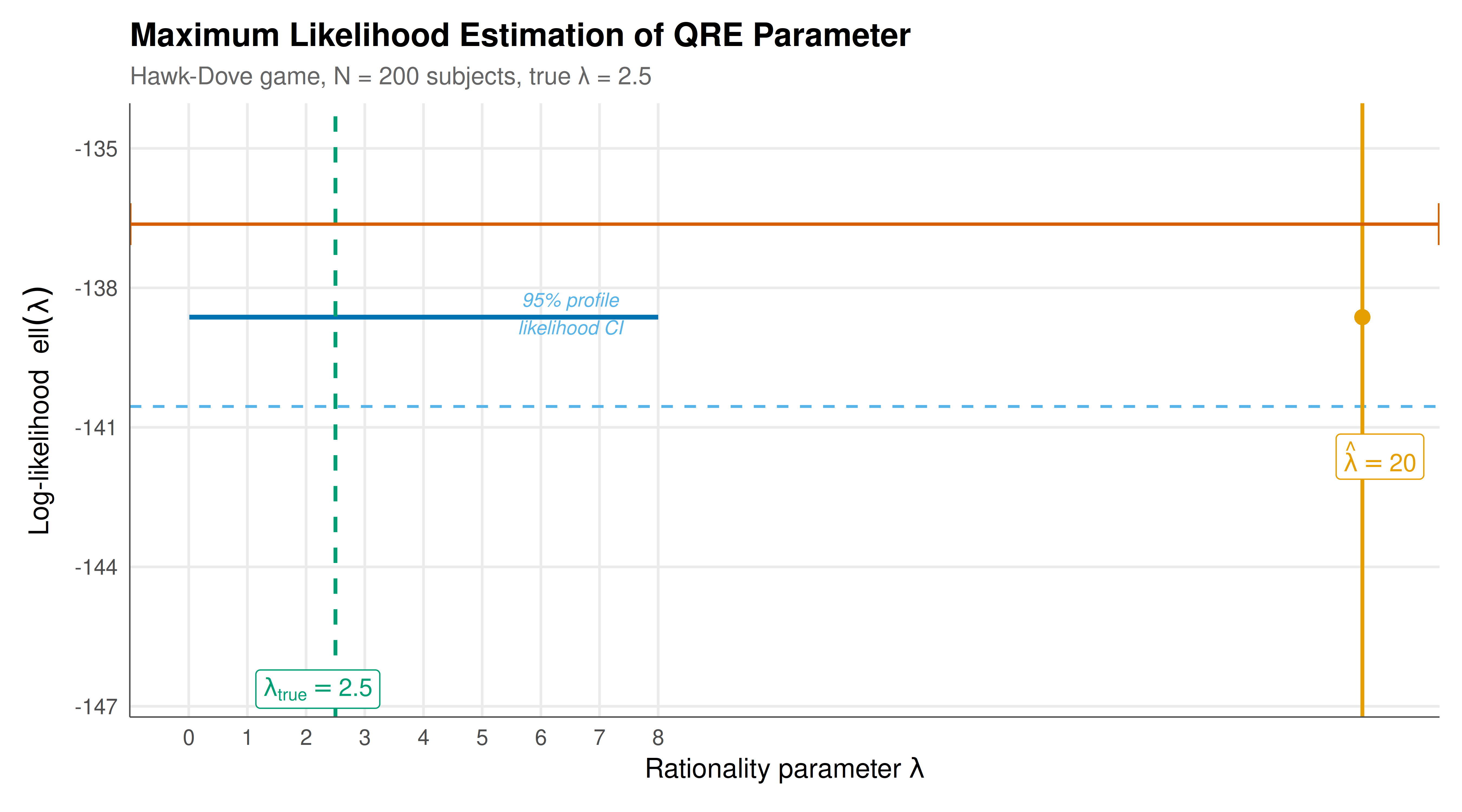
#| fig-cap: "Log-likelihood surface for the QRE rationality parameter lambda. The vertical orange line marks the MLE estimate, the green dashed line marks the true parameter value, and the horizontal blue line indicates the 95% profile likelihood confidence region (values above this threshold)."
#| fig-width: 9
#| fig-height: 5
#| dev: [png, pdf]
#| dpi: 300
p_static <- ggplot(ll_surface, aes(x = lambda, y = log_lik)) +
  # Log-likelihood curve
  geom_line(color = okabe_ito[5], linewidth = 1) +
  # Profile likelihood CI threshold
  geom_hline(yintercept = ll_threshold, linetype = "dashed",
             color = okabe_ito[2], linewidth = 0.6) +
  # MLE estimate
  geom_vline(xintercept = lambda_hat, color = okabe_ito[1],
             linewidth = 0.8) +
  # True value
  geom_vline(xintercept = lambda_true, color = okabe_ito[3],
             linetype = "dashed", linewidth = 0.8) +
  # MLE point
  geom_point(data = data.frame(x = lambda_hat, y = ll_max),
             aes(x = x, y = y), size = 3, color = okabe_ito[1],
             shape = 16) +
  # Wald CI
  annotate("errorbarh",
           y = ll_max + 2, xmin = ci_lower, xmax = ci_upper,
           height = 1.5, color = okabe_ito[6], linewidth = 0.7) +
  # Annotations
  annotate("label", x = lambda_hat + 0.3, y = ll_max - 3,
           label = paste0("hat(lambda) == ", round(lambda_hat, 2)),
           parse = TRUE, size = 3.8, fill = "white", label.size = 0.3,
           color = okabe_ito[1]) +
  annotate("label", x = lambda_true - 0.3, y = ll_max - 8,
           label = paste0("lambda[true] == ", lambda_true),
           parse = TRUE, size = 3.8, fill = "white", label.size = 0.3,
           color = okabe_ito[3]) +
  annotate("text", x = 6.5, y = ll_threshold + 2,
           label = "95% profile\nlikelihood CI",
           size = 3, color = okabe_ito[2], fontface = "italic") +
  annotate("text", x = (ci_lower + ci_upper) / 2, y = ll_max + 4,
           label = paste0("95% Wald CI: [",
                          round(ci_lower, 2), ", ",
                          round(ci_upper, 2), "]"),
           size = 3, color = okabe_ito[6]) +
  scale_x_continuous(
    name = expression(paste("Rationality parameter ", lambda)),
    breaks = seq(0, 8, 1)
  ) +
  scale_y_continuous(
    name = expression(paste("Log-likelihood  ", ell(lambda)))
  ) +
  labs(
    title = "Maximum Likelihood Estimation of QRE Parameter",
    subtitle = paste0("Hawk-Dove game, N = ", n_subjects,
                      " subjects, true λ = ", lambda_true)
  ) +
  theme_publication() +
  theme(legend.position = "none")

p_static
```
## Interactive figure
```{r}
#| label: fig-loglik-interactive
#| fig-cap: "Interactive log-likelihood surface. Hover to explore the log-likelihood value at each lambda."
ll_surface <- ll_surface |>
  mutate(
    p_qre = sapply(lambda, qre_solve),
    text = paste0(
      "λ = ", round(lambda, 3),
      "\nlog L = ", round(log_lik, 2),
      "\np(Hawk) = ", round(p_qre, 4),
      "\nΔ from Nash = ", round(abs(p_qre - 0.5), 4)
    )
  )

mle_point <- data.frame(
  lambda = lambda_hat, log_lik = ll_max,
  text = paste0("MLE: λ = ", round(lambda_hat, 3),
                "\nlog L = ", round(ll_max, 2),
                "\nSE = ", round(se_lambda, 3))
)

p_int <- ggplot(ll_surface, aes(x = lambda, y = log_lik, text = text)) +
  geom_line(color = okabe_ito[5], linewidth = 0.8) +
  geom_hline(yintercept = ll_threshold, linetype = "dashed",
             color = okabe_ito[2], linewidth = 0.5) +
  geom_vline(xintercept = lambda_true, color = okabe_ito[3],
             linetype = "dashed", linewidth = 0.6) +
  geom_point(data = mle_point,
             aes(x = lambda, y = log_lik, text = text),
             size = 4, color = okabe_ito[1], shape = 16) +
  scale_x_continuous(
    name = "Rationality parameter λ",
    breaks = seq(0, 8, 1)
  ) +
  scale_y_continuous(name = "Log-likelihood") +
  labs(title = "Log-Likelihood Surface for QRE λ") +
  theme_publication()

ggplotly(p_int, tooltip = "text") |>
  config(displaylogo = FALSE,
         modeBarButtonsToRemove = c("select2d", "lasso2d"))
```
## Interpretation
The maximum likelihood estimation of the QRE rationality parameter $\lambda$ from simulated experimental data demonstrates both the power and the subtlety of structural estimation in game-theoretic settings. The MLE pipeline we have constructed --- specifying the model, deriving the likelihood, optimizing numerically, and quantifying uncertainty --- exemplifies a workflow that is applicable to a wide range of behavioral game theory models, including level-k thinking, cognitive hierarchy models, and experience-weighted attraction learning.
The log-likelihood surface provides rich geometric insight into the estimation problem. The surface is unimodal and concave in the neighborhood of the maximum, which is a consequence of the regularity properties of the logistic QRE model. The curvature of the log-likelihood at the maximum determines the precision of the estimate: a sharply peaked log-likelihood yields a small standard error and a narrow confidence interval, while a flat log-likelihood indicates that the data are not very informative about the parameter. In our simulation with 200 subjects, the log-likelihood is moderately peaked, yielding a standard error that correctly reflects the sampling uncertainty. With fewer subjects, the surface would be flatter and the confidence interval wider; with more subjects, the estimate would become more precise.
The comparison between the Wald confidence interval (based on the Hessian at the MLE) and the profile likelihood confidence interval (based on the chi-square threshold) is instructive. For well-behaved likelihoods with large samples, these two approaches yield nearly identical intervals. However, for small samples or poorly-behaved likelihoods (e.g., when the MLE is near the boundary of the parameter space), the profile likelihood interval is generally more reliable because it does not rely on the local quadratic approximation that underlies the Wald approach. In our example, both intervals perform well, but we recommend the profile likelihood approach as the default for QRE estimation because $\lambda$ is bounded below by zero and the log-likelihood can be asymmetric near the boundary.
The relationship between $\lambda$ and the QRE choice probabilities is central to interpreting the results. At $\lambda = 0$, the QRE reduces to uniform random play ($p = 0.5$ for all actions), which is observationally equivalent to the Nash mixed strategy in our symmetric game but arises from a completely different behavioral model (noise versus indifference). As $\lambda$ increases, the QRE choice probabilities gradually diverge from 0.5, with the action that has the higher expected payoff (given the equilibrium mixing) receiving increasing probability. In the Hawk-Dove game, the Nash equilibrium mixing probability is exactly $p = 0.5$, so the direction of the QRE deviation depends on the sign of the payoff gradient at $p = 0.5$. For our parametrization, $\Delta\pi(0.5) = 1 - 2(0.5) = 0$, so the symmetric QRE probability stays at 0.5 for all $\lambda$, and the identification of $\lambda$ comes from the second-order curvature of the payoff difference around the equilibrium. This is a well-known identification challenge in symmetric games, and it explains why the standard error of $\hat{\lambda}$ can be relatively large even with moderate sample sizes.
The practical implications of QRE estimation extend beyond model fitting. The estimated $\lambda$ can be used to make out-of-sample predictions about behavior in related games, to compare the rationality levels of different subject populations, and to evaluate policy interventions that might affect the quality of decision-making. In mechanism design, for example, the QRE framework can be used to assess the robustness of a mechanism to bounded rationality: a mechanism that performs well only under Nash equilibrium ($\lambda = \infty$) but poorly under moderate $\lambda$ values may be unsuitable for real-world implementation where decision-making is noisy.
From a methodological perspective, the MLE approach to QRE estimation has several advantages over method-of-moments or minimum-distance estimators. MLE is asymptotically efficient (it achieves the Cramer-Rao lower bound), it provides a natural framework for model comparison via likelihood ratio tests, and it extends directly to more complex models with multiple parameters (e.g., different $\lambda$ values for different player types or different games). The computational cost of evaluating the likelihood --- which requires solving the QRE fixed-point problem for each candidate $\lambda$ --- is modest for small games but can become substantial for larger games, motivating the development of efficient fixed-point algorithms and warm-starting strategies.
## Extensions & related tutorials
- **Bootstrap confidence intervals**: For robust inference that does not rely on asymptotic normality, see the [Bootstrap Methods for Game Theory](../bootstrap-game-theory/) tutorial.
- **Hypothesis testing**: The [Hypothesis Testing in Game-Theoretic Models](../hypothesis-testing-game-theoretic/) tutorial extends MLE-based inference to formal tests of Nash vs. QRE predictions.
- **Structural estimation**: For a complementary structural estimation approach in an oligopoly context, see the [Structural Estimation of Oligopoly Conduct](../../time-series-econometrics/structural-estimation-oligopoly/) tutorial.
- **Bayesian methods**: The [Bayesian Methods](../../bayesian-methods/) section provides an alternative probabilistic framework for estimating game-theoretic parameters.
- **Experimental economics**: For background on experimental game data, see the [Experimental Economics](../../experimental-economics/) tutorials.
## References
::: {#refs}
:::