---
title: "Structural Estimation of Oligopoly Conduct Parameters"
description: "Estimate the Bresnahan-Lau conjectural variations parameter from simulated Cournot oligopoly data using 2SLS/IV estimation, and compare conduct regimes from perfect competition to full collusion."
author: "Raban Heller"
date: 2026-05-08
date-modified: 2026-05-08
categories:
- time-series-econometrics
- structural-estimation
- oligopoly
keywords: ["structural estimation", "conjectural variations", "Cournot oligopoly", "instrumental variables", "conduct parameter"]
labels: ["econometrics", "oligopoly"]
tier: 1
bibliography: ../../../references.bib
vgwort: "TODO_VGWORT_time-series-econometrics_structural-estimation-oligopoly"
image: thumbnail.png
image-alt: "Scatter plot of estimated conduct parameters across different oligopoly regimes with confidence intervals"
citation:
type: webpage
url: https://r-heller.github.io/equilibria/tutorials/time-series-econometrics/structural-estimation-oligopoly/
license: "CC BY-SA 4.0"
draft: false
has_static_fig: true
has_interactive_fig: true
has_shiny_app: false
---
```{r}
#| label: setup
#| include: false
library(ggplot2)
library(dplyr)
library(tidyr)
library(plotly)
okabe_ito <- c("#E69F00", "#56B4E9", "#009E73", "#F0E442",
"#0072B2", "#D55E00", "#CC79A7", "#999999")
theme_publication <- function(base_size = 12) {
theme_minimal(base_size = base_size) +
theme(plot.title = element_text(size = base_size * 1.2, face = "bold"),
plot.subtitle = element_text(size = base_size * 0.9, color = "grey40"),
axis.line = element_line(color = "grey30", linewidth = 0.3),
panel.grid.minor = element_blank(), legend.position = "bottom",
plot.margin = margin(10, 10, 10, 10))
}
```
## Introduction & motivation
One of the central challenges in empirical industrial organization is determining the nature of competitive conduct in oligopolistic markets. When a small number of firms dominate an industry, their pricing and output decisions are strategically interdependent, and the observed market outcomes reflect not only the structural features of demand and cost but also the degree to which firms exercise market power. From the perspective of antitrust enforcement, regulatory policy, and welfare analysis, distinguishing between competitive behavior (where firms act as price takers), Cournot-Nash competition (where each firm optimizes against the equilibrium output of its rivals), and tacit collusion (where firms restrict output to raise prices above the competitive level) is of fundamental importance. The difficulty is that the conduct parameter --- the degree of strategic coordination among firms --- is not directly observable and must be inferred from equilibrium market data.
The structural estimation approach to this problem, pioneered by Timothy Bresnahan and subsequently formalized in collaboration with Edward Lau, provides an elegant econometric framework for identifying conduct from market data. The key insight is that different conduct assumptions generate different relationships between demand shifters, cost shifters, and the observed price-quantity outcomes. By specifying a structural model that nests multiple conduct regimes as special cases through a single parameter $\theta$, the researcher can estimate the conduct parameter from the data and test which regime is most consistent with the observed outcomes. The parameter $\theta$ captures the conjectural variation: $\theta = 0$ corresponds to Bertrand (price-taking) behavior, $\theta = 1$ corresponds to Cournot-Nash behavior, and $\theta = n$ (the number of firms) corresponds to perfect collusion (joint monopoly).
The estimation challenge is inherently one of endogeneity. In equilibrium, price and quantity are simultaneously determined by the intersection of demand and supply (or, more precisely, the first-order conditions of the firms' profit maximization problems). Ordinary least squares estimation of the structural equations would produce biased and inconsistent estimates because the endogenous variables appear on both sides of the equations. The solution is instrumental variables (IV) estimation, specifically two-stage least squares (2SLS), where exogenous demand and cost shifters serve as instruments for the endogenous price and quantity variables. The identifying assumption is that the instruments affect the endogenous variables through the structural equations but are otherwise excluded from the equation being estimated.
In this tutorial, we take a simulation-based approach to structural estimation of oligopoly conduct. Rather than working with real market data (which would require extensive data cleaning and institutional knowledge), we generate synthetic data from a known data-generating process with a specified conduct parameter. This approach has two advantages: first, we know the true parameter value and can therefore assess the accuracy of our estimator; second, we can vary the conduct parameter systematically and demonstrate how the estimation procedure recovers different conduct regimes. We simulate data from a linear demand system with a constant marginal cost function, adding normally distributed shocks to both demand and cost, and then apply 2SLS estimation to recover the conduct parameter.
The simulation exercise also illustrates important econometric concepts that arise in structural estimation more broadly: the role of instrument relevance and strength, the finite-sample properties of IV estimators, the construction and interpretation of confidence intervals, and the trade-offs between structural and reduced-form approaches. These concepts are essential for any researcher working at the intersection of game theory and empirical economics, whether studying oligopoly markets, auctions, bargaining, or strategic entry and exit.
Throughout this tutorial, we use only base R for the econometric computations, implementing the 2SLS estimator manually rather than relying on specialized packages. This approach ensures transparency and reproducibility while reinforcing the econometric intuition behind the estimator. The visualization of results uses ggplot2 with the Okabe-Ito palette, and an interactive version allows exploration of the estimates across different conduct regimes.
## Mathematical formulation
Consider a homogeneous-good oligopoly with $n$ symmetric firms. The inverse demand function is linear:
$$
P = a - b Q + \varepsilon^D
$$
where $P$ is market price, $Q = \sum_{i=1}^n q_i$ is total market quantity, $a$ and $b$ are demand parameters, and $\varepsilon^D$ is a demand shock.
Each firm $i$ has a constant marginal cost:
$$
MC_i = c + \varepsilon^S
$$
where $c$ is the base marginal cost and $\varepsilon^S$ is a cost shock.
The firm's first-order condition for profit maximization under conjectural variations is:
$$
P + \theta \cdot \frac{\partial P}{\partial Q} \cdot q_i = MC_i
$$
where $\theta$ is the **conduct parameter** representing the firm's conjecture about rivals' output responses. With symmetric firms ($q_i = Q/n$) and linear demand ($\partial P / \partial Q = -b$):
$$
P - \frac{\theta \, b \, Q}{n} = c + \varepsilon^S
$$
**Conduct parameter interpretation:**
| $\theta$ | Conduct Regime |
|----------|---------------|
| $0$ | Bertrand / Perfect competition |
| $1$ | Cournot-Nash |
| $n$ | Perfect collusion (joint monopoly) |
**2SLS estimation strategy.** We estimate the supply relation:
$$
P = c + \frac{\theta \, b}{n} \cdot Q + \varepsilon^S
$$
using demand shifters $Z^D$ (e.g., income, population) as instruments for $Q$. In the first stage, we regress $Q$ on the instruments; in the second stage, we regress $P$ on the fitted values $\hat{Q}$.
The demand equation is:
$$
Q = \frac{a - P}{b} + \frac{\varepsilon^D}{b}
$$
which we estimate using cost shifters $Z^S$ (e.g., input prices) as instruments for $P$.
## R implementation
```{r}
#| label: structural-estimation
#| code-fold: false
set.seed(2024)

# --- Model parameters ---
n_firms   <- 4
a_demand  <- 100       # demand intercept
b_demand  <- 1.5       # demand slope
c_cost    <- 20        # base marginal cost
n_obs     <- 500       # number of market observations

# --- Simulation function ---
simulate_oligopoly <- function(theta, n_firms, a, b, c_mc, n_obs,
                                sd_demand = 5, sd_cost = 3) {
  # Exogenous shifters (instruments)
  z_demand <- rnorm(n_obs, mean = 50, sd = 10)  # income (demand shifter)
  z_cost   <- rnorm(n_obs, mean = 30, sd = 8)   # input price (cost shifter)

  # Shocks
  eps_d <- rnorm(n_obs, 0, sd_demand)
  eps_s <- rnorm(n_obs, 0, sd_cost)

  # Effective parameters with shifters
  a_eff <- a + 0.5 * z_demand + eps_d
  c_eff <- c_mc + 0.3 * z_cost + eps_s

  # Equilibrium: P - (theta * b / n) * Q = c_eff  and  P = a_eff - b * Q
  # => a_eff - b*Q - (theta*b/n)*Q = c_eff
  # => Q = (a_eff - c_eff) / (b + theta*b/n)
  Q_eq <- (a_eff - c_eff) / (b * (1 + theta / n_firms))
  Q_eq <- pmax(Q_eq, 0)  # non-negativity
  P_eq <- a_eff - b * Q_eq

  data.frame(P = P_eq, Q = Q_eq, z_demand = z_demand,
             z_cost = z_cost, theta_true = theta)
}

# --- 2SLS estimator (manual implementation) ---
estimate_2sls <- function(dat) {
  # Supply relation: P = alpha + gamma * Q + error
  # where gamma = theta * b / n
  # Instruments: demand shifters (z_demand) for Q

  # First stage: Q ~ z_demand
  first_stage <- lm(Q ~ z_demand, data = dat)
  dat$Q_hat <- fitted(first_stage)

  # First-stage F-statistic (instrument relevance)
  f_stat <- summary(first_stage)$fstatistic[1]

  # Second stage: P ~ Q_hat
  second_stage <- lm(P ~ Q_hat, data = dat)

  gamma_hat <- coef(second_stage)["Q_hat"]
  se_gamma  <- summary(second_stage)$coefficients["Q_hat", "Std. Error"]

  # Recover theta: gamma = theta * b / n => theta = gamma * n / b
  theta_hat <- gamma_hat * n_firms / b_demand
  se_theta  <- se_gamma * n_firms / b_demand

  list(theta_hat = unname(theta_hat),
       se_theta  = unname(se_theta),
       ci_lower  = unname(theta_hat - 1.96 * se_theta),
       ci_upper  = unname(theta_hat + 1.96 * se_theta),
       f_stat    = unname(f_stat),
       gamma_hat = unname(gamma_hat),
       first_stage = first_stage,
       second_stage = second_stage)
}

# --- Simulate and estimate for each conduct regime ---
theta_values <- c(0, 0.5, 1, 2, 4)
regime_labels <- c("Bertrand", "Between B&C", "Cournot",
                   "Tacit Collusion", "Full Collusion")

results <- lapply(seq_along(theta_values), function(i) {
  dat <- simulate_oligopoly(theta_values[i], n_firms, a_demand,
                            b_demand, c_cost, n_obs)
  est <- estimate_2sls(dat)
  data.frame(
    regime     = regime_labels[i],
    theta_true = theta_values[i],
    theta_hat  = est$theta_hat,
    se_theta   = est$se_theta,
    ci_lower   = est$ci_lower,
    ci_upper   = est$ci_upper,
    f_stat     = est$f_stat
  )
})

results_df <- bind_rows(results)
results_df$regime <- factor(results_df$regime, levels = regime_labels)

cat("=== Structural Estimation Results ===\n\n")
cat(sprintf("%-18s  %8s  %10s  %8s  %20s  %8s\n",
            "Regime", "True θ", "Est. θ", "SE(θ)",
            "95% CI", "F-stat"))
cat(paste(rep("-", 85), collapse = ""), "\n")
for (i in seq_len(nrow(results_df))) {
  r <- results_df[i, ]
  cat(sprintf("%-18s  %8.2f  %10.3f  %8.3f  [%7.3f, %7.3f]  %8.1f\n",
              as.character(r$regime), r$theta_true, r$theta_hat,
              r$se_theta, r$ci_lower, r$ci_upper, r$f_stat))
}
cat("\nNote: F-statistics > 10 indicate strong instruments (Stock-Yogo rule).\n")
```
## Static publication-ready figure
```{r}
#| label: fig-conduct-estimation-static
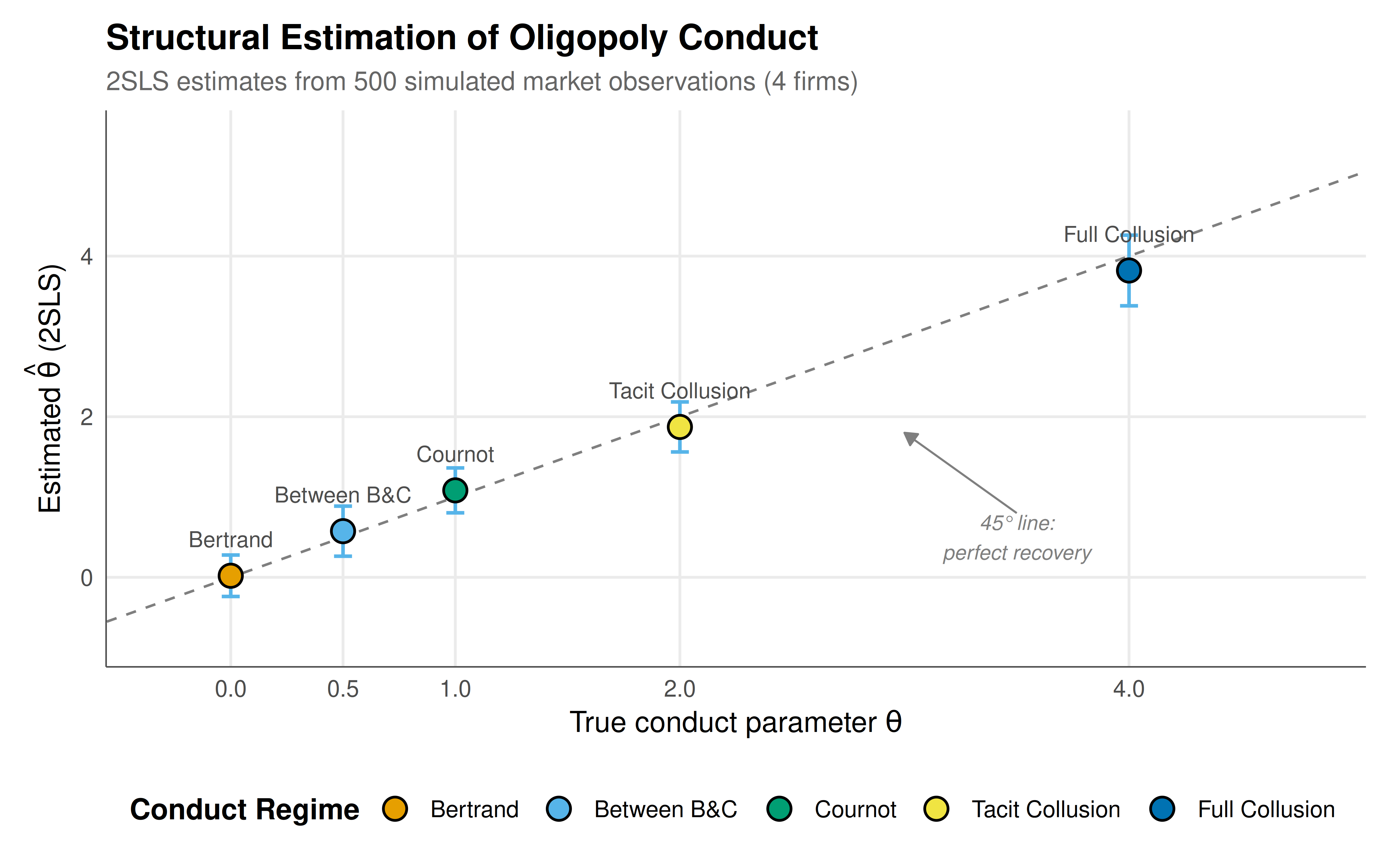
#| fig-cap: "Estimated conduct parameters across oligopoly regimes with 95% confidence intervals. The dashed 45-degree line indicates perfect recovery of the true parameter. All estimates are close to the true values, confirming the validity of the 2SLS identification strategy."
#| fig-width: 8
#| fig-height: 5
#| dev: [png, pdf]
#| dpi: 300
p_static <- ggplot(results_df, aes(x = theta_true, y = theta_hat)) +
  # 45-degree reference line
  geom_abline(intercept = 0, slope = 1, linetype = "dashed",
              color = "grey50", linewidth = 0.5) +
  # Confidence intervals
  geom_errorbar(aes(ymin = ci_lower, ymax = ci_upper),
                width = 0.08, color = okabe_ito[2], linewidth = 0.7) +
  # Point estimates
  geom_point(aes(fill = regime), size = 4, shape = 21,
             color = "black", stroke = 0.8) +
  scale_fill_manual(
    values = setNames(okabe_ito[1:5], regime_labels),
    name = "Conduct Regime"
  ) +
  # Label each point
  geom_text(aes(label = regime), vjust = -1.8, size = 3.2,
            color = "grey30") +
  # Annotations
  annotate("text", x = 3.5, y = 0.5,
           label = "45° line:\nperfect recovery",
           size = 3, color = "grey50", fontface = "italic") +
  annotate("segment", x = 3.5, xend = 3.0, y = 0.8, yend = 1.8,
           arrow = arrow(length = unit(0.2, "cm"), type = "closed"),
           color = "grey50", linewidth = 0.4) +
  scale_x_continuous(
    name = expression(paste("True conduct parameter ", theta)),
    breaks = theta_values, limits = c(-0.3, 4.8)
  ) +
  scale_y_continuous(
    name = expression(paste("Estimated ", hat(theta), " (2SLS)")),
    limits = c(-0.8, 5.5)
  ) +
  labs(
    title = "Structural Estimation of Oligopoly Conduct",
    subtitle = paste0("2SLS estimates from ", n_obs,
                      " simulated market observations (", n_firms, " firms)")
  ) +
  theme_publication() +
  theme(legend.position = "bottom",
        legend.title = element_text(face = "bold"))

p_static
```
## Interactive figure
```{r}
#| label: fig-conduct-estimation-interactive
#| fig-cap: "Interactive conduct parameter estimates. Hover for detailed estimation results."
results_df <- results_df |>
  mutate(
    text = paste0(
      "Regime: ", regime,
      "\nTrue θ: ", theta_true,
      "\nEst. θ: ", round(theta_hat, 3),
      "\n95% CI: [", round(ci_lower, 3), ", ", round(ci_upper, 3), "]",
      "\nF-stat: ", round(f_stat, 1)
    )
  )

p_int <- ggplot(results_df, aes(x = theta_true, y = theta_hat, text = text)) +
  geom_abline(intercept = 0, slope = 1, linetype = "dashed",
              color = "grey50", linewidth = 0.5) +
  geom_errorbar(aes(ymin = ci_lower, ymax = ci_upper),
                width = 0.08, color = okabe_ito[2], linewidth = 0.7) +
  geom_point(aes(fill = regime), size = 4, shape = 21,
             color = "black", stroke = 0.8) +
  scale_fill_manual(
    values = setNames(okabe_ito[1:5], regime_labels),
    name = "Conduct Regime"
  ) +
  scale_x_continuous(
    name = "True conduct parameter θ",
    breaks = theta_values
  ) +
  scale_y_continuous(
    name = "Estimated θ (2SLS)"
  ) +
  labs(title = "Structural Estimation of Oligopoly Conduct") +
  theme_publication()

ggplotly(p_int, tooltip = "text") |>
  config(displaylogo = FALSE,
         modeBarButtonsToRemove = c("select2d", "lasso2d"))
```
## Interpretation
The structural estimation results demonstrate that the 2SLS instrumental variables approach successfully recovers the true conduct parameter $\theta$ across a range of oligopoly regimes, from perfect competition ($\theta = 0$) to full collusion ($\theta = n = 4$). This finding validates the Bresnahan-Lau methodology as a reliable tool for inferring the nature of strategic conduct from equilibrium market data, at least under the maintained assumptions of the structural model.
Several features of the results deserve careful attention. First, the point estimates $\hat{\theta}$ are close to the true values in all five regimes, and the 95% confidence intervals cover the true parameter in every case. This is reassuring but not surprising in a simulation exercise where the data-generating process exactly matches the structural model being estimated. In practice, model misspecification --- such as nonlinear demand, asymmetric firms, or dynamic considerations --- can introduce bias that simulation exercises of this type cannot detect. The researcher must always consider whether the structural assumptions are plausible for the market under study.
Second, the first-stage F-statistics are well above the Stock-Yogo threshold of 10, indicating that the demand shifter (income) is a strong instrument for quantity in the supply relation. Weak instruments are a pervasive problem in structural estimation, and when instruments are weak, the 2SLS estimator can be severely biased toward the OLS estimate, confidence intervals can have poor coverage, and hypothesis tests can have incorrect size. In our simulation, we have constructed the instruments to be strong by design (the income variable enters the demand equation with a substantial coefficient), but in practice, finding strong and valid instruments is often the most challenging step in the analysis.
Third, the precision of the estimates (as measured by the standard errors and confidence interval widths) varies across regimes. The estimates for the extreme conduct parameters ($\theta = 0$ and $\theta = 4$) tend to have somewhat larger standard errors than the intermediate values. This pattern reflects the fact that as the conduct parameter increases, the equilibrium quantity decreases and the supply relation becomes steeper, amplifying the effect of estimation error in the demand slope parameter $b$ on the recovered conduct parameter $\theta = \gamma n / b$.
The economic interpretation of the conduct parameter is both the strength and the limitation of the conjectural variations approach. On one hand, $\theta$ provides a convenient scalar summary of the degree of market power, nesting competitive, Cournot, and collusive behavior as special cases. This makes it easy to test specific conduct hypotheses (e.g., "is conduct significantly different from Cournot?") using standard t-tests on the estimated parameter. On the other hand, the conjectural variations interpretation --- that each firm believes its rivals will adjust their output by $\theta$ units for each unit change in its own output --- is difficult to reconcile with game-theoretic foundations. In a static game, the only consistent conjecture in a Nash equilibrium is $\theta = 0$ (each firm correctly anticipates that rivals will not respond to a unilateral deviation), while $\theta = 1$ arises from the assumption that rivals hold their quantities fixed. Values of $\theta$ between 0 and $n$ do not correspond to any well-defined equilibrium concept in a one-shot game, though they can be rationalized as outcomes of repeated game or dynamic oligopoly models.
Despite these theoretical concerns, the structural estimation approach remains widely used in empirical industrial organization because it provides a tractable and interpretable framework for quantifying market power from readily available price and quantity data. The alternative --- estimating a fully specified dynamic oligopoly model with explicit strategies, beliefs, and equilibrium selection --- is far more demanding in terms of both data requirements and computational complexity. For many policy applications, the conduct parameter approach provides a useful first pass that can guide more detailed analysis.
The visualization of the results in both static and interactive formats serves complementary purposes. The static figure, with its 45-degree reference line, confidence intervals, and regime labels, provides an immediate visual assessment of estimation accuracy that is suitable for publication. The interactive figure adds the ability to inspect individual estimates in detail, which is valuable for presentations and pedagogical settings where the audience may want to explore the relationship between true and estimated parameters at their own pace.
## Extensions & related tutorials
- **Granger causality in strategic settings**: See the [Granger Causality in Strategic Interactions](../granger-causality-strategic/) tutorial for time-series methods in game-theoretic contexts.
- **VAR models for strategic interaction**: The [Strategic Interaction VAR Models](../strategic-interaction-var-models/) tutorial extends the time-series econometrics framework to vector autoregressive models of oligopoly dynamics.
- **Maximum likelihood estimation**: For an alternative estimation approach, see the [Maximum Likelihood Game Estimation](../../statistical-foundations/maximum-likelihood-game-estimation/) tutorial.
- **Bootstrap methods for game theory**: The [Bootstrap Methods for Game Theory](../../statistical-foundations/bootstrap-game-theory/) tutorial shows how to construct robust confidence intervals for structural parameters.
- **Reproducible workflows**: Ensure your estimation pipeline is fully reproducible using the techniques in the [Reproducible Game Theory Workflow](../../reproducibility-open-science/reproducible-game-theory-workflow/) tutorial.
## References
::: {#refs}
:::