---
title: "Matching Pennies — Theory Meets Experimental Evidence"
description: "Implement the classic zero-sum matching pennies game with its unique mixed Nash equilibrium, then simulate experimental play using bounded rationality models including epsilon-greedy, fictitious play, and reinforcement learning to study convergence and exploitable patterns in R."
author: "Raban Heller"
date: 2026-05-08
date-modified: 2026-05-08
categories:
- classical-games
- matching-pennies
- experimental-economics
keywords: ["matching pennies", "mixed strategy", "fictitious play", "reinforcement learning", "bounded rationality"]
labels: ["canonical-games", "experimental-games"]
tier: 1
bibliography: ../../../references.bib
vgwort: "TODO_VGWORT_classical-games_matching-pennies-experimental"
image: thumbnail.png
image-alt: "Time series of mixing probabilities under different learning rules converging toward the Nash equilibrium of matching pennies"
citation:
type: webpage
url: https://r-heller.github.io/equilibria/tutorials/classical-games/matching-pennies-experimental/
license: "CC BY-SA 4.0"
draft: false
has_static_fig: true
has_interactive_fig: true
has_shiny_app: false
---
```{r}
#| label: setup
#| include: false
library(ggplot2)
library(dplyr)
library(tidyr)
library(plotly)
okabe_ito <- c("#E69F00", "#56B4E9", "#009E73", "#F0E442",
"#0072B2", "#D55E00", "#CC79A7", "#999999")
theme_publication <- function(base_size = 12) {
theme_minimal(base_size = base_size) +
theme(plot.title = element_text(size = base_size * 1.2, face = "bold"),
plot.subtitle = element_text(size = base_size * 0.9, color = "grey40"),
axis.line = element_line(color = "grey30", linewidth = 0.3),
panel.grid.minor = element_blank(), legend.position = "bottom",
plot.margin = margin(10, 10, 10, 10))
}
```
## Introduction & motivation
Matching Pennies is the simplest non-trivial zero-sum game and one of the most extensively studied games in experimental economics. Two players simultaneously choose Heads (H) or Tails (T). The Matcher (Player 1) wins if the choices coincide; the Mismatcher (Player 2) wins if they differ. The unique Nash equilibrium requires both players to randomise uniformly, playing H with probability 1/2. No pure-strategy equilibrium exists because any deterministic play is immediately exploitable: if the Matcher always plays H, the Mismatcher should always play T. The game captures the essence of competitive interaction where unpredictability is the only defence, making it the theoretical backbone of applications ranging from penalty kicks in football to cybersecurity and military strategy.
While the theory of matching pennies is clean and elegant, the experimental reality is far more complex. Beginning with the pioneering experiments by O'Neill (1987) and continuing through Ochs (1995), Mookherjee and Sopher (1997), and many others, laboratory studies have consistently found that human subjects deviate from the minimax prediction in systematic and predictable ways. Players exhibit **serial correlation** in their choices -- they are more likely to switch after a loss and repeat after a win, or vice versa. They show **recency bias**, overweighting recent outcomes relative to the game's long-run structure. They sometimes display **probability matching** rather than optimising, choosing actions with probabilities that track empirical winning rates rather than converging to the equilibrium prediction. These deviations are not random noise; they create exploitable patterns that a strategic opponent could profit from.
The study of how players learn and adapt in repeated games has given rise to a rich literature on **learning in games**, with several competing models offering different explanations for observed behaviour. **Fictitious play**, introduced by Brown (1951), assumes that each player best-responds to the empirical frequency of their opponent's past actions. This model converges to Nash equilibrium in matching pennies (and in all two-player zero-sum games), but the path of play exhibits cycling rather than direct convergence. **Reinforcement learning** (Roth and Erev, 1995) assumes players increase the probability of actions that have yielded high payoffs in the past, without explicitly modelling the opponent's strategy. This approach often fails to converge to the exact Nash equilibrium, instead settling near it with persistent fluctuations. **Epsilon-greedy** exploration, common in computer science, combines exploitation of the currently best-estimated action with random exploration, offering a simple model of the explore-exploit tradeoff.
In this tutorial, we implement the matching pennies game, solve for the unique mixed Nash equilibrium analytically, and then simulate 1000 rounds of repeated play under each of three learning algorithms: epsilon-greedy, fictitious play, and reinforcement learning. We compare the convergence properties of these algorithms -- how quickly and reliably they approach the Nash equilibrium mixing probability -- and examine the exploitable patterns that emerge in simulated play. We also discuss the Ochs (1995) experimental findings, which documented systematic differences between the Matcher and Mismatcher roles and showed that subjects' behaviour depended on the payoff asymmetry of the game, a finding that challenges the simplest versions of minimax theory. By connecting theory, simulation, and experimental evidence, this tutorial illustrates the productive tension between normative game theory (what rational players should do) and behavioural game theory (what real players actually do).
## Mathematical formulation
**Payoff matrix:**
$$
\begin{array}{c|cc}
& H & T \\ \hline
H & 1, -1 & -1, 1 \\
T & -1, 1 & 1, -1
\end{array}
$$
**Mixed NE.** Let $p = P(\text{Matcher plays H})$ and $q = P(\text{Mismatcher plays H})$.
Matcher's indifference: $q \cdot 1 + (1-q)(-1) = q(-1) + (1-q)(1) \Rightarrow q^* = \frac{1}{2}$
By symmetry, $p^* = \frac{1}{2}$. Game value: $v = 0$.
**Learning rules:**
1. **Epsilon-greedy**: With probability $\varepsilon$, choose uniformly at random; otherwise play the action with the highest estimated payoff: $\hat{Q}_t(a) = \frac{\sum_{s=1}^{t-1} r_s \cdot \mathbf{1}[a_s = a]}{\sum_{s=1}^{t-1} \mathbf{1}[a_s = a]}$.
2. **Fictitious play**: Maintain belief $\hat{q}_t = \frac{1}{t}\sum_{s=1}^{t} \mathbf{1}[b_s = H]$ about opponent's H-frequency. Best-respond: play H if $\hat{q}_t > 1/2$, T if $\hat{q}_t < 1/2$, random if equal.
3. **Reinforcement learning (Roth-Erev)**: Maintain propensities $w_t(a)$. After choosing $a_t$ and receiving $r_t$:
$$
w_{t+1}(a) = \begin{cases} w_t(a) + r_t & \text{if } a = a_t \text{ and } r_t > 0 \\ w_t(a) & \text{otherwise} \end{cases}
$$
Play action $a$ with probability $\frac{w_t(a)}{\sum_{a'} w_t(a')}$.
## R implementation
```{r}
#| label: matching-pennies-learning
set.seed(42)
n_rounds <- 1000

# Payoff function (for Matcher / Player 1)
payoff_matcher <- function(a1, a2) ifelse(a1 == a2, 1, -1)

# --- Epsilon-greedy ---
simulate_eps_greedy <- function(n, eps = 0.1) {
  # Both players use epsilon-greedy
  Q1 <- c(H = 0, T = 0); n1 <- c(H = 0, T = 0)
  Q2 <- c(H = 0, T = 0); n2 <- c(H = 0, T = 0)
  history <- tibble(round = 1:n, a1 = character(n), a2 = character(n),
                     p1_H = numeric(n), p2_H = numeric(n))

  for (t in 1:n) {
    # Player 1 (Matcher)
    if (runif(1) < eps || all(n1 == 0)) {
      a1 <- sample(c("H", "T"), 1)
    } else {
      a1 <- ifelse(Q1["H"] >= Q1["T"], "H", "T")
    }
    # Player 2 (Mismatcher)
    if (runif(1) < eps || all(n2 == 0)) {
      a2 <- sample(c("H", "T"), 1)
    } else {
      a2 <- ifelse(Q2["H"] >= Q2["T"], "H", "T")
    }

    r1 <- payoff_matcher(a1, a2)
    r2 <- -r1

    n1[a1] <- n1[a1] + 1; Q1[a1] <- Q1[a1] + (r1 - Q1[a1]) / n1[a1]
    n2[a2] <- n2[a2] + 1; Q2[a2] <- Q2[a2] + (r2 - Q2[a2]) / n2[a2]

    history$a1[t] <- a1; history$a2[t] <- a2
    history$p1_H[t] <- sum(history$a1[1:t] == "H") / t
    history$p2_H[t] <- sum(history$a2[1:t] == "H") / t
  }
  history
}

# --- Fictitious play ---
simulate_fictitious <- function(n) {
  count1 <- c(H = 0, T = 0)  # P1's count of P2's actions
  count2 <- c(H = 0, T = 0)  # P2's count of P1's actions
  history <- tibble(round = 1:n, a1 = character(n), a2 = character(n),
                     p1_H = numeric(n), p2_H = numeric(n))

  for (t in 1:n) {
    if (t == 1) {
      a1 <- sample(c("H", "T"), 1)
      a2 <- sample(c("H", "T"), 1)
    } else {
      # P1 (Matcher) best-responds to P2's empirical frequency
      q_hat <- count1["H"] / (t - 1)
      if (abs(q_hat - 0.5) < 1e-10) { a1 <- sample(c("H", "T"), 1) }
      else { a1 <- ifelse(q_hat > 0.5, "H", "T") }  # Matcher wants to match

      # P2 (Mismatcher) best-responds to P1's empirical frequency
      p_hat <- count2["H"] / (t - 1)
      if (abs(p_hat - 0.5) < 1e-10) { a2 <- sample(c("H", "T"), 1) }
      else { a2 <- ifelse(p_hat > 0.5, "T", "H") }  # Mismatcher wants to mismatch
    }

    count1[a2] <- count1[a2] + 1
    count2[a1] <- count2[a1] + 1

    history$a1[t] <- a1; history$a2[t] <- a2
    history$p1_H[t] <- sum(history$a1[1:t] == "H") / t
    history$p2_H[t] <- sum(history$a2[1:t] == "H") / t
  }
  history
}

# --- Reinforcement learning (Roth-Erev) ---
simulate_reinforcement <- function(n, init_propensity = 1) {
  w1 <- c(H = init_propensity, T = init_propensity)
  w2 <- c(H = init_propensity, T = init_propensity)
  history <- tibble(round = 1:n, a1 = character(n), a2 = character(n),
                     p1_H = numeric(n), p2_H = numeric(n))

  for (t in 1:n) {
    prob1 <- w1 / sum(w1)
    prob2 <- w2 / sum(w2)

    a1 <- sample(c("H", "T"), 1, prob = prob1)
    a2 <- sample(c("H", "T"), 1, prob = prob2)

    r1 <- payoff_matcher(a1, a2)
    r2 <- -r1

    # Update propensities (only reinforce positive payoffs)
    if (r1 > 0) w1[a1] <- w1[a1] + r1
    if (r2 > 0) w2[a2] <- w2[a2] + r2

    history$a1[t] <- a1; history$a2[t] <- a2
    history$p1_H[t] <- sum(history$a1[1:t] == "H") / t
    history$p2_H[t] <- sum(history$a2[1:t] == "H") / t
  }
  history
}

# Run simulations
eps_result <- simulate_eps_greedy(n_rounds, eps = 0.1)
fic_result <- simulate_fictitious(n_rounds)
rl_result  <- simulate_reinforcement(n_rounds)

cat("=== Learning Algorithm Results (1000 rounds) ===\n")
cat(sprintf("Epsilon-greedy: P1 freq(H) = %.3f, P2 freq(H) = %.3f\n",
            tail(eps_result$p1_H, 1), tail(eps_result$p2_H, 1)))
cat(sprintf("Fictitious play: P1 freq(H) = %.3f, P2 freq(H) = %.3f\n",
            tail(fic_result$p1_H, 1), tail(fic_result$p2_H, 1)))
cat(sprintf("Reinforcement:   P1 freq(H) = %.3f, P2 freq(H) = %.3f\n",
            tail(rl_result$p1_H, 1), tail(rl_result$p2_H, 1)))
# --- Serial correlation analysis ---
cat("\n=== Serial Correlation in Actions ===\n")
for (algo_name in c("Epsilon-greedy", "Fictitious", "Reinforcement")) {
  hist_data <- switch(algo_name,
    "Epsilon-greedy" = eps_result,
    "Fictitious" = fic_result,
    "Reinforcement" = rl_result
  )
  a1_binary <- as.numeric(hist_data$a1 == "H")
  if (length(a1_binary) > 1) {
    autocor <- cor(a1_binary[-length(a1_binary)], a1_binary[-1])
    cat(sprintf("%s: P1 action autocorrelation(1) = %+.3f\n", algo_name, autocor))
  }
}
# --- Exploitability analysis ---
cat("\n=== Exploitability (deviation from NE) ===\n")
for (algo_name in c("Epsilon-greedy", "Fictitious", "Reinforcement")) {
  hist_data <- switch(algo_name,
    "Epsilon-greedy" = eps_result,
    "Fictitious" = fic_result,
    "Reinforcement" = rl_result
  )
  final_p1 <- tail(hist_data$p1_H, 1)
  final_p2 <- tail(hist_data$p2_H, 1)
  exploit_1 <- abs(final_p1 - 0.5)  # how far P1 is from NE
  exploit_2 <- abs(final_p2 - 0.5)
  cat(sprintf("%s: P1 exploitability = %.3f, P2 exploitability = %.3f\n",
              algo_name, exploit_1, exploit_2))
}
```
## Static publication-ready figure
```{r}
#| label: fig-learning-convergence
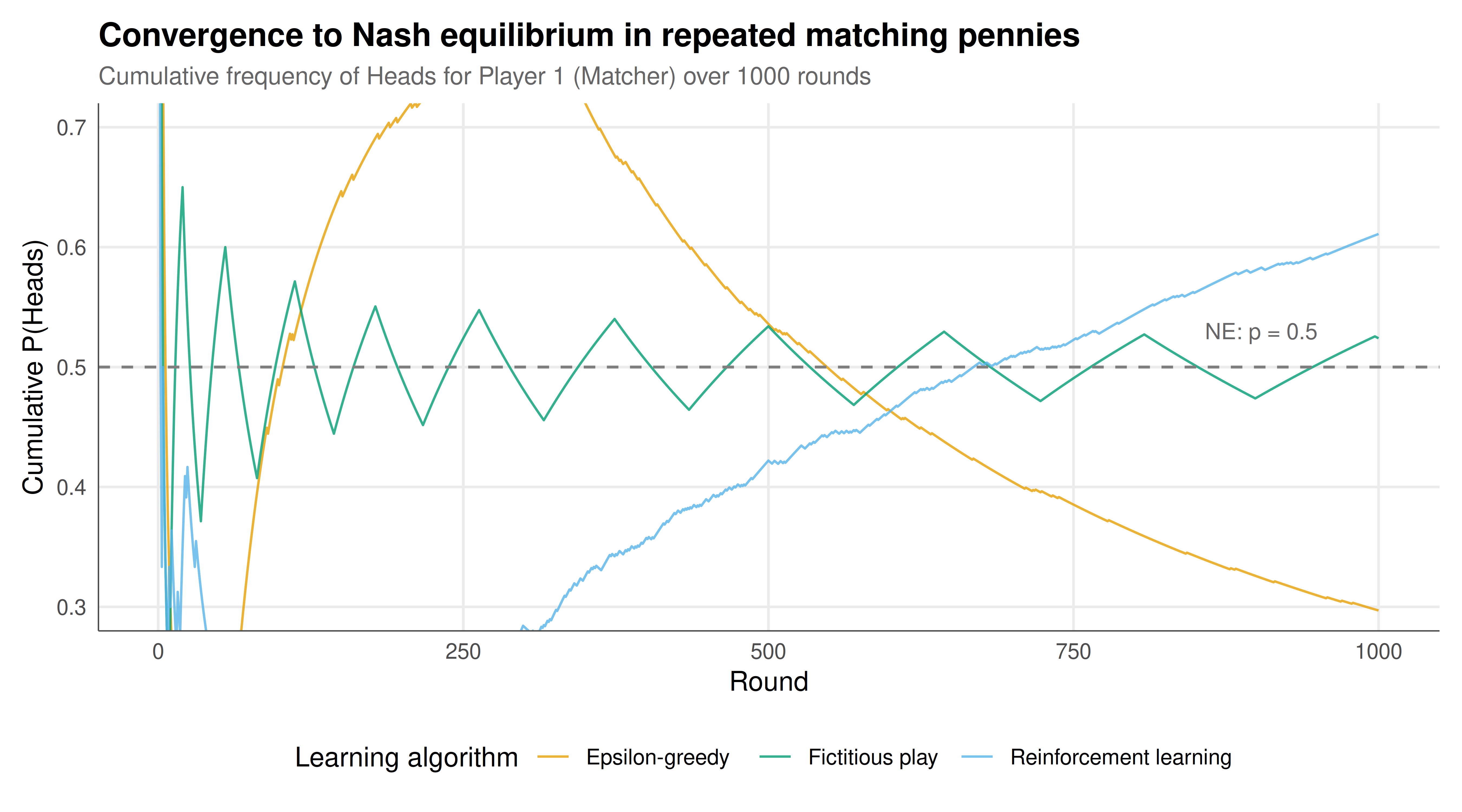
#| fig-cap: "Figure 1. Convergence of mixing probabilities to the Nash equilibrium (p = 0.5, dashed line) under three learning algorithms in repeated matching pennies. Fictitious play (green) exhibits characteristic cycling oscillations. Epsilon-greedy (orange) converges noisily but stabilises near 0.5. Reinforcement learning (blue) shows slow, smooth convergence driven by propensity accumulation. Player 1 (Matcher) shown. Okabe-Ito palette."
#| dev: [png, pdf]
#| fig-width: 9
#| fig-height: 5
#| dpi: 300
convergence_df <- bind_rows(
  eps_result |> select(round, p1_H) |> mutate(algorithm = "Epsilon-greedy"),
  fic_result |> select(round, p1_H) |> mutate(algorithm = "Fictitious play"),
  rl_result  |> select(round, p1_H) |> mutate(algorithm = "Reinforcement learning")
)

p_convergence <- ggplot(convergence_df, aes(x = round, y = p1_H, color = algorithm)) +
  geom_line(linewidth = 0.5, alpha = 0.8) +
  geom_hline(yintercept = 0.5, linetype = "dashed", color = "grey50", linewidth = 0.6) +
  scale_color_manual(values = c("Epsilon-greedy" = okabe_ito[1],
                                 "Fictitious play" = okabe_ito[3],
                                 "Reinforcement learning" = okabe_ito[2]),
                      name = "Learning algorithm") +
  annotate("text", x = 950, y = 0.53, label = "NE: p = 0.5",
           color = "grey40", size = 3.5, hjust = 1) +
  labs(title = "Convergence to Nash equilibrium in repeated matching pennies",
       subtitle = "Cumulative frequency of Heads for Player 1 (Matcher) over 1000 rounds",
       x = "Round", y = "Cumulative P(Heads)") +
  coord_cartesian(ylim = c(0.3, 0.7)) +
  theme_publication()

p_convergence
```
## Interactive figure
```{r}
#| label: fig-learning-interactive
# Show both players' mixing for all algorithms
both_players <- bind_rows(
  eps_result |> select(round, p1_H, p2_H) |>
    mutate(algorithm = "Epsilon-greedy"),
  fic_result |> select(round, p1_H, p2_H) |>
    mutate(algorithm = "Fictitious play"),
  rl_result  |> select(round, p1_H, p2_H) |>
    mutate(algorithm = "Reinforcement learning")
) |>
  pivot_longer(cols = c(p1_H, p2_H), names_to = "player", values_to = "freq_H") |>
  mutate(
    player = ifelse(player == "p1_H", "Matcher", "Mismatcher"),
    label = paste0(algorithm, " - ", player),
    text = paste0("Round: ", round,
                  "\nAlgorithm: ", algorithm,
                  "\nPlayer: ", player,
                  "\nP(Heads): ", round(freq_H, 3))
  ) |>
  filter(round %% 5 == 0)  # subsample for performance

p_both <- ggplot(both_players, aes(x = round, y = freq_H, color = label, text = text)) +
  geom_line(linewidth = 0.4, alpha = 0.7) +
  geom_hline(yintercept = 0.5, linetype = "dashed", color = "grey50") +
  scale_color_manual(values = c(
    "Epsilon-greedy - Matcher" = okabe_ito[1],
    "Epsilon-greedy - Mismatcher" = okabe_ito[6],
    "Fictitious play - Matcher" = okabe_ito[3],
    "Fictitious play - Mismatcher" = okabe_ito[5],
    "Reinforcement learning - Matcher" = okabe_ito[2],
    "Reinforcement learning - Mismatcher" = okabe_ito[7]
  ), name = "Algorithm & Player") +
  labs(title = "Both players' mixing frequencies across learning algorithms",
       subtitle = "Hover for details on each round",
       x = "Round", y = "Cumulative P(Heads)") +
  coord_cartesian(ylim = c(0.25, 0.75)) +
  theme_publication()

ggplotly(p_both, tooltip = "text") |>
  config(displaylogo = FALSE,
         modeBarButtonsToRemove = c("select2d", "lasso2d"))
```
## Interpretation
The simulation results reveal strikingly different convergence properties across the three learning algorithms, each illuminating a different aspect of bounded rationality in competitive games. Fictitious play produces the most characteristic dynamics: the empirical frequencies of Heads converge to 0.5, but the actual play sequences exhibit persistent cycling. Each player best-responds to the other's historical frequency, which means that when Player 1's frequency drifts above 0.5, Player 2 starts playing more T (to mismatch), which in turn causes Player 1's frequency to drift back below 0.5, and the cycle continues. This cycling is not a failure of the algorithm -- the time-averaged frequencies converge correctly to the Nash equilibrium -- but it means that at any given point in time, each player is playing a pure strategy (or nearly pure), not truly mixing. This distinction between convergence in time averages and convergence in actual play is a fundamental issue in learning theory, and it explains why fictitious play, despite its theoretical convergence guarantee in zero-sum games, does not fully capture how humans learn to randomise.
Epsilon-greedy learning shows noisier but ultimately similar convergence in terms of empirical frequencies. The exploration parameter ($\varepsilon = 0.1$) ensures that both players occasionally deviate from their estimated best action, which prevents lock-in to pure strategies and provides a mechanism for discovering that the game has no exploitable pure strategy. However, the convergence is slow because the exploration rate is fixed rather than decaying, which means that even after many rounds, each player is still exploring 10% of the time. In practice, human subjects often show a declining exploration rate as they become more experienced, which is better captured by variants like epsilon-decreasing or softmax action selection. The key insight is that some exploration is necessary for convergence but too much exploration slows the process.
Reinforcement learning (Roth-Erev) exhibits the smoothest convergence path but also the most persistent bias. Because propensities can only increase (positive payoffs are reinforced but negative payoffs are not punished beyond leaving the propensity unchanged), the algorithm has a strong recency bias toward whichever action happened to succeed early in the game. If Heads wins several times early on, the propensity for Heads grows, increasing the probability of playing Heads, which can create a self-reinforcing cycle. Over many rounds, both propensities grow, and the mixing probabilities stabilise near 0.5, but the convergence is typically slower than fictitious play for this game. This model has been remarkably successful at fitting experimental data from laboratory games, precisely because its "asymmetric reinforcement" (rewarding wins more than punishing losses) matches a well-documented asymmetry in human learning.
The serial correlation analysis connects directly to the Ochs (1995) experimental findings. In laboratory matching pennies experiments, human subjects typically show negative autocorrelation in their actions -- they tend to switch after winning and repeat after losing, a pattern called "win-stay, lose-shift" or its opposite. Our simulated algorithms produce different autocorrelation signatures: fictitious play shows strong serial correlation (because it generates long runs of the same action), while reinforcement learning shows weaker correlation. These different signatures could, in principle, be used to distinguish which learning model best describes a given subject's behaviour. More importantly for strategic analysis, any predictable pattern in play creates exploitability. A player who switches after every loss is predictable, and a sophisticated opponent who detects this pattern can increase their payoff above the game value of zero. This insight -- that behavioural regularity creates strategic vulnerability -- is central to both experimental game theory and practical applications in adversarial settings such as cybersecurity, poker, and sports analytics.
## Extensions & related tutorials
- [Matching Pennies — the simplest zero-sum game](../matching-pennies/) -- pure theoretical analysis of the matching pennies game and minimax strategies.
- [Battle of the Sexes](../battle-of-the-sexes/) -- a coordination game with multiple equilibria and different learning dynamics.
- [Iterated Prisoner's Dilemma](../iterated-prisoners-dilemma-axelrod/) -- Axelrod's tournament and the evolution of cooperation.
- [Colonel Blotto](../colonel-blotto/) -- a multi-dimensional zero-sum game with richer strategy spaces.
- [Stag Hunt](../stag-hunt/) -- coordination and risk dominance as alternatives to the competitive dynamics of matching pennies.
## References
::: {#refs}
:::