---
title: "The Allais paradox and expected utility violations"
description: "Demonstrate the Allais paradox as a systematic violation of the independence axiom in expected utility theory, implement EU calculations in R, and explore prospect theory's probability weighting as an explanation."
author: "Raban Heller"
date: 2026-05-08
date-modified: 2026-05-08
categories:
- decision-theory
- allais-paradox
- expected-utility
- prospect-theory
keywords: ["Allais paradox", "expected utility", "independence axiom", "probability weighting", "prospect theory", "risk preference", "Marschak-Machina triangle"]
labels: ["decision-theory", "behavioural-anomalies"]
tier: 1
bibliography: ../../../references.bib
vgwort: "TODO_VGWORT_decision-theory_allais-paradox"
image: thumbnail.png
image-alt: "Marschak-Machina probability triangle showing Allais-type choice patterns violating the independence axiom"
citation:
type: webpage
url: https://r-heller.github.io/equilibria/tutorials/decision-theory/allais-paradox/
license: "CC BY-SA 4.0"
draft: false
has_static_fig: true
has_interactive_fig: true
has_shiny_app: false
---
```{r}
#| label: setup
#| include: false
library(ggplot2)
library(dplyr)
library(tidyr)
library(plotly)
okabe_ito <- c("#E69F00", "#56B4E9", "#009E73", "#F0E442",
"#0072B2", "#D55E00", "#CC79A7", "#999999")
theme_publication <- function(base_size = 12) {
theme_minimal(base_size = base_size) +
theme(
plot.title = element_text(size = base_size * 1.2, face = "bold"),
plot.subtitle = element_text(size = base_size * 0.9, color = "grey40"),
axis.line = element_line(color = "grey30", linewidth = 0.3),
panel.grid.minor = element_blank(),
legend.position = "bottom",
plot.margin = margin(10, 10, 10, 10)
)
}
```
## Introduction & motivation
In 1953, the French economist Maurice Allais presented a pair of choice problems to a distinguished audience at a conference in Paris. Among those present was Leonard Savage, the architect of subjective expected utility theory, who himself fell into the "trap" that Allais had set. The Allais paradox, as it came to be known, demonstrates that the **independence axiom** -- the central axiom distinguishing expected utility from mere ordinal preference -- is systematically violated by most people's choices. This was not a minor empirical curiosity: it struck at the foundations of the decision theory that underpins virtually all of economics and game theory.
The paradox consists of two choice problems. In the first (the "common consequence" problem), subjects choose between a certain gain of one million francs and a gamble offering a 10% chance of five million, an 89% chance of one million, and a 1% chance of nothing. Most people prefer the certainty. In the second problem, subjects choose between an 11% chance of one million (and 89% chance of nothing) and a 10% chance of five million (and 90% chance of nothing). Most people prefer the second gamble. The crucial insight is that these two preference patterns together are **inconsistent with any expected utility function**: the common consequence of 89% probability of one million has been replaced by 89% probability of nothing in both options of the second problem, and the independence axiom requires that this replacement should not reverse the preference. Yet it systematically does.
The Allais paradox has had profound consequences for economic theory. It motivated the development of **non-expected utility theories**, most notably Kahneman and Tversky's prospect theory (1979, 1992), which explains the Allais pattern through two psychological mechanisms: **probability weighting** (people overweight small probabilities and underweight large ones) and **loss aversion**. The probability weighting function $w(p)$ is concave for small $p$ (overweighting) and convex for large $p$ (underweighting), producing the characteristic inverse-S shape. Applied to the Allais problems, this weighting naturally generates the observed choice pattern without any contradiction because probability weighting explicitly relaxes the independence axiom.
This tutorial implements the expected utility calculations demonstrating the inconsistency, visualises the choice problems in the Marschak-Machina probability triangle (which provides geometric intuition for why independence fails), simulates a heterogeneous population to estimate the prevalence of Allais-type violations, and compares the predictions of EU theory with those of rank-dependent utility and cumulative prospect theory.
## Mathematical formulation
Consider lotteries over three outcomes: $0$ (nothing), $M$ (one million), and $5M$ (five million). A lottery is a probability vector $(p_0, p_M, p_{5M})$ with $p_0 + p_M + p_{5M} = 1$.
**Problem 1** (common consequence):
- Lottery A: $(0, 1, 0)$ -- certainty of $M$
- Lottery B: $(0.01, 0.89, 0.10)$ -- risky gamble
**Problem 2** (common ratio):
- Lottery C: $(0.89, 0.11, 0)$ -- 11% chance of $M$
- Lottery D: $(0.90, 0, 0.10)$ -- 10% chance of $5M$
Under expected utility $U(L) = p_0 u(0) + p_M u(M) + p_{5M} u(5M)$, normalise $u(0) = 0$, $u(M) = 1$, and let $u(5M) = v$.
$$
A \succ B \iff 1 > 0.89 + 0.10v \iff v < 1.1
$$
$$
D \succ C \iff 0.10v > 0.11 \iff v > 1.1
$$
These conditions are **contradictory**: $v < 1.1$ and $v > 1.1$ cannot both hold. The modal choice pattern $A \succ B$ and $D \succ C$ violates EU for **any** utility function.
**Independence axiom violation**: Transform Problem 1 to Problem 2 by replacing the common consequence (89% chance of $M$) with 89% chance of $0$:
$$
A' = 0.11 \cdot (0, 1, 0) + 0.89 \cdot (1, 0, 0) = C
$$
$$
B' = 0.11 \cdot (0.01/0.11, 0, 0.10/0.11) + 0.89 \cdot (1, 0, 0) = D
$$
Independence requires: $A \succ B \Rightarrow C \succ D$. But the modal preference reverses.
**Prospect theory explanation**: Under cumulative prospect theory with probability weighting function $w(p) = \frac{p^\gamma}{(p^\gamma + (1-p)^\gamma)^{1/\gamma}}$ (Tversky-Kahneman, $\gamma \approx 0.65$), the certainty of A receives full weight while B's 1% chance of zero is overweighted, making A attractive. In Problem 2, neither option offers certainty, and the overweighting of the 10% chance of $5M$ in D makes it attractive.
## R implementation
```{r}
#| label: allais-analysis
# Expected utility calculations
allais_eu <- function(v, u0 = 0, uM = 1) {
  # v = u(5M) / u(M) relative utility of 5M
  # Problem 1
  eu_A <- uM  # certainty of M
  eu_B <- 0.01 * u0 + 0.89 * uM + 0.10 * (v * uM)  # risky gamble

  # Problem 2
  eu_C <- 0.89 * u0 + 0.11 * uM
  eu_D <- 0.90 * u0 + 0.10 * (v * uM)

  list(eu_A = eu_A, eu_B = eu_B, eu_C = eu_C, eu_D = eu_D,
       pref1 = ifelse(eu_A > eu_B, "A", "B"),
       pref2 = ifelse(eu_C > eu_D, "C", "D"))
}

cat("=== Allais Paradox: EU Analysis ===\n")
cat("\nFor different values of u(5M)/u(M):\n")
for (v in c(0.5, 1.0, 1.05, 1.1, 1.15, 1.5, 2.0, 3.0)) {
  result <- allais_eu(v)
  cat(sprintf("  v = %.2f: EU(A)=%.3f, EU(B)=%.3f -> %s | EU(C)=%.3f, EU(D)=%.3f -> %s",
              v, result$eu_A, result$eu_B, result$pref1,
              result$eu_C, result$eu_D, result$pref2))
  consistent <- (result$pref1 == "A" & result$pref2 == "C") |
                (result$pref1 == "B" & result$pref2 == "D")
  cat(ifelse(consistent, " [EU consistent]\n", " [VIOLATES EU]\n"))
}
cat("\nCritical value: v = 1.1 is the boundary.\n")
cat("A > B requires v < 1.1; D > C requires v > 1.1.\n")
cat("Modal choice (A, D) is impossible under ANY EU function.\n")
# Probability weighting function (Tversky-Kahneman)
pw_tk <- function(p, gamma = 0.65) {
  p^gamma / (p^gamma + (1 - p)^gamma)^(1/gamma)
}

# Rank-dependent utility with probability weighting
rdu_value <- function(outcomes, probs, u_func, gamma = 0.65) {
  # Sort outcomes in increasing order
  ord <- order(outcomes)
  outcomes <- outcomes[ord]
  probs <- probs[ord]

  # Cumulative probabilities
  cum_probs <- cumsum(probs)
  cum_probs_prev <- c(0, cum_probs[-length(cum_probs)])

  # Decision weights
  weights <- pw_tk(cum_probs, gamma) - pw_tk(cum_probs_prev, gamma)

  sum(weights * u_func(outcomes))
}

u_func <- function(x) x^0.5  # Concave utility (risk averse)

cat("\n=== Rank-Dependent Utility (gamma = 0.65) ===\n")
rdu_A <- rdu_value(c(1), c(1), u_func)
rdu_B <- rdu_value(c(0, 1, 5), c(0.01, 0.89, 0.10), u_func)
rdu_C <- rdu_value(c(0, 1), c(0.89, 0.11), u_func)
rdu_D <- rdu_value(c(0, 5), c(0.90, 0.10), u_func)

cat(sprintf("RDU(A) = %.4f, RDU(B) = %.4f -> Prefer %s\n",
            rdu_A, rdu_B, ifelse(rdu_A > rdu_B, "A", "B")))
cat(sprintf("RDU(C) = %.4f, RDU(D) = %.4f -> Prefer %s\n",
            rdu_C, rdu_D, ifelse(rdu_C > rdu_D, "C", "D")))
cat(sprintf("Pattern: (%s, %s) — %s\n",
            ifelse(rdu_A > rdu_B, "A", "B"),
            ifelse(rdu_C > rdu_D, "C", "D"),
            ifelse((rdu_A > rdu_B) & (rdu_D > rdu_C), "Allais pattern!", "No violation")))
# Simulate heterogeneous population
cat("\n=== Population Simulation: 10000 agents ===\n")
set.seed(42)
n_agents <- 10000
gammas <- runif(n_agents, 0.3, 1.0)  # Heterogeneous probability weighting
alphas <- runif(n_agents, 0.3, 0.9)  # Heterogeneous risk aversion (u(x) = x^alpha)

agent_choices <- sapply(1:n_agents, function(i) {
  u_i <- function(x) x^alphas[i]
  g_i <- gammas[i]

  rdu_Ai <- rdu_value(c(1), c(1), u_i, g_i)
  rdu_Bi <- rdu_value(c(0, 1, 5), c(0.01, 0.89, 0.10), u_i, g_i)
  rdu_Ci <- rdu_value(c(0, 1), c(0.89, 0.11), u_i, g_i)
  rdu_Di <- rdu_value(c(0, 5), c(0.90, 0.10), u_i, g_i)

  c(ifelse(rdu_Ai > rdu_Bi, "A", "B"), ifelse(rdu_Ci > rdu_Di, "C", "D"))
})

choice_patterns <- table(
  Problem1 = agent_choices[1, ],
  Problem2 = agent_choices[2, ]
)
cat("Choice pattern frequencies:\n")
print(choice_patterns)
cat(sprintf("\nAllais pattern (A, D): %.1f%%\n",
            100 * sum(agent_choices[1,] == "A" & agent_choices[2,] == "D") / n_agents))
cat(sprintf("EU-consistent (A, C): %.1f%%\n",
            100 * sum(agent_choices[1,] == "A" & agent_choices[2,] == "C") / n_agents))
cat(sprintf("EU-consistent (B, D): %.1f%%\n",
            100 * sum(agent_choices[1,] == "B" & agent_choices[2,] == "D") / n_agents))
cat(sprintf("Reverse Allais (B, C): %.1f%%\n",
            100 * sum(agent_choices[1,] == "B" & agent_choices[2,] == "C") / n_agents))
```
## Static publication-ready figure
```{r}
#| label: fig-allais-triangle
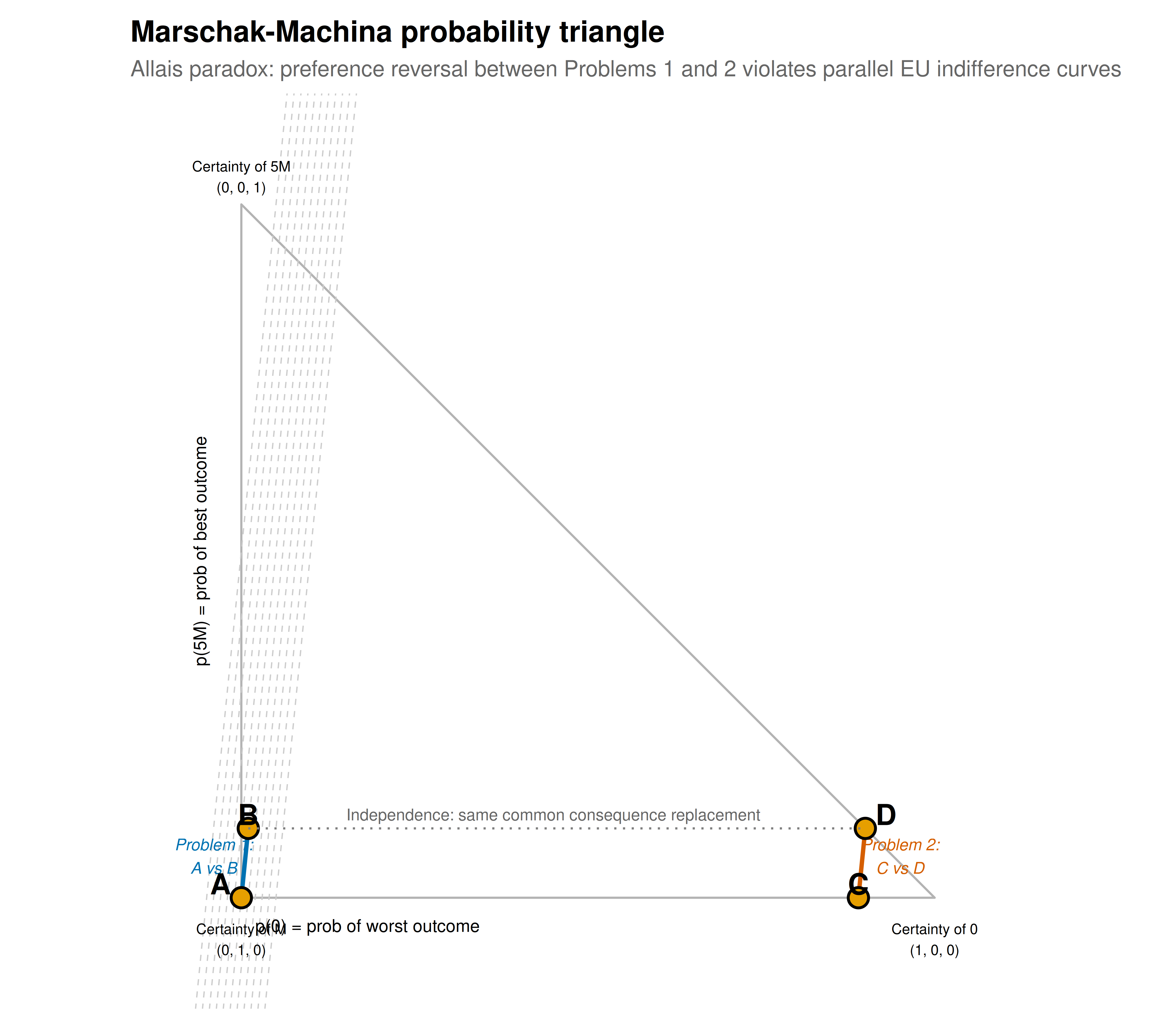
#| fig-cap: "Figure 1. Marschak-Machina probability triangle for the Allais paradox. The axes represent probabilities of the worst outcome (p0, horizontal) and best outcome (p5M, vertical), with the probability of the middle outcome determined by the constraint p0 + pM + p5M = 1. Lotteries A, B, C, D are plotted as points. Under EU theory, indifference curves are parallel straight lines (grey dashed). The Allais pattern (A preferred to B, D preferred to C) requires indifference curves that fan out (steeper near the certainty axis), which is exactly what probability weighting produces. Okabe-Ito palette."
#| dev: [png, pdf]
#| fig-width: 8
#| fig-height: 7
#| dpi: 300
# Marschak-Machina triangle: axes are p0 (prob of 0) and p5M (prob of 5M)
# p_M = 1 - p0 - p5M

# Lottery coordinates: (p0, p5M)
lotteries <- tibble(
  name = c("A", "B", "C", "D"),
  p0 = c(0, 0.01, 0.89, 0.90),
  p5M = c(0, 0.10, 0, 0.10),
  label_x = c(-0.03, 0.01, 0.89, 0.93),
  label_y = c(0.02, 0.12, 0.02, 0.12)
)

# EU indifference curves: u(0)p0 + u(M)(1-p0-p5M) + u(5M)p5M = k
# Rearranging: p5M = (k - u(M) + (u(M) - u(0))p0) / (u(5M) - u(M))
# These are parallel lines with slope (u(M) - u(0)) / (u(5M) - u(M))

# EU indifference curves for v = 1.1
v <- 1.1
slope_eu <- 1 / (v - 1)  # = 10 for v = 1.1

eu_lines <- tibble(
  intercept = seq(-0.5, 0.5, by = 0.1),
  slope = slope_eu
)

p_triangle <- ggplot() +
  # Triangle boundary
  annotate("polygon", x = c(0, 1, 0, 0), y = c(0, 0, 1, 0),
           fill = NA, color = "grey70", linewidth = 0.5) +
  # EU indifference curves (parallel lines)
  geom_abline(data = eu_lines, aes(intercept = intercept, slope = slope),
              color = "grey80", linetype = "dashed", linewidth = 0.3) +
  # Problem 1 connection (A-B)
  annotate("segment", x = 0, y = 0, xend = 0.01, yend = 0.10,
           color = okabe_ito[5], linewidth = 1, arrow = arrow(length = unit(0.15, "cm"))) +
  annotate("text", x = -0.04, y = 0.06, label = "Problem 1:\nA vs B",
           size = 2.8, color = okabe_ito[5], fontface = "italic") +
  # Problem 2 connection (C-D)
  annotate("segment", x = 0.89, y = 0, xend = 0.90, yend = 0.10,
           color = okabe_ito[6], linewidth = 1, arrow = arrow(length = unit(0.15, "cm"))) +
  annotate("text", x = 0.95, y = 0.06, label = "Problem 2:\nC vs D",
           size = 2.8, color = okabe_ito[6], fontface = "italic") +
  # Lottery points
  geom_point(data = lotteries, aes(x = p0, y = p5M),
             size = 4, shape = 21, fill = okabe_ito[1], color = "black", stroke = 1) +
  geom_text(data = lotteries, aes(x = label_x, y = label_y, label = name),
            size = 5, fontface = "bold") +
  # Independence axiom direction
  annotate("segment", x = 0.01, y = 0.10, xend = 0.90, yend = 0.10,
           color = "grey50", linetype = "dotted", linewidth = 0.5) +
  annotate("text", x = 0.45, y = 0.12,
           label = "Independence: same common consequence replacement",
           size = 2.8, color = "grey40") +
  # Certainty line
  annotate("text", x = 0.02, y = -0.04, label = "p(0) = prob of worst outcome",
           size = 3, hjust = 0) +
  annotate("text", x = -0.06, y = 0.5, label = "p(5M) = prob of best outcome",
           size = 3, angle = 90) +
  # Corner labels
  annotate("text", x = 0, y = -0.06, label = "Certainty of M\n(0, 1, 0)",
           size = 2.5, hjust = 0.5) +
  annotate("text", x = 1, y = -0.06, label = "Certainty of 0\n(1, 0, 0)",
           size = 2.5, hjust = 0.5) +
  annotate("text", x = 0, y = 1.04, label = "Certainty of 5M\n(0, 0, 1)",
           size = 2.5, hjust = 0.5) +
  coord_fixed(xlim = c(-0.1, 1.1), ylim = c(-0.1, 1.1)) +
  labs(
    title = "Marschak-Machina probability triangle",
    subtitle = "Allais paradox: preference reversal between Problems 1 and 2 violates parallel EU indifference curves"
  ) +
  theme_publication() +
  theme(
    axis.text = element_blank(),
    axis.title = element_blank(),
    panel.grid.major = element_blank(),
    axis.line = element_blank()
  )

p_triangle
```
## Interactive figure
```{r}
#| label: fig-allais-weighting
# Probability weighting functions for different gamma values
p_grid <- seq(0.001, 0.999, by = 0.005)
gamma_vals <- c(0.50, 0.65, 0.80, 1.00)

pw_data <- bind_rows(lapply(gamma_vals, function(g) {
  tibble(
    p = p_grid,
    wp = pw_tk(p_grid, g),
    gamma = g,
    gamma_label = sprintf("gamma = %.2f", g),
    text = paste0("p = ", round(p_grid, 3),
                  "\nw(p) = ", round(pw_tk(p_grid, g), 3),
                  "\ngamma = ", g,
                  ifelse(g == 1, " (EU: no distortion)", ""))
  )
}))

pw_data$gamma_label <- factor(pw_data$gamma_label,
                                levels = sprintf("gamma = %.2f", gamma_vals))

p_weighting <- ggplot(pw_data, aes(x = p, y = wp, color = gamma_label, text = text)) +
  geom_line(linewidth = 1) +
  geom_abline(slope = 1, intercept = 0, linetype = "dashed", color = "grey60") +
  scale_color_manual(values = okabe_ito[c(6, 1, 2, 8)],
                      name = "Weighting parameter") +
  # Mark key probabilities from Allais problems
  annotate("point", x = 0.01, y = pw_tk(0.01, 0.65), size = 3, color = okabe_ito[6]) +
  annotate("text", x = 0.01, y = pw_tk(0.01, 0.65) + 0.05,
           label = "1% overweighted", size = 2.5, hjust = 0) +
  annotate("point", x = 0.89, y = pw_tk(0.89, 0.65), size = 3, color = okabe_ito[6]) +
  annotate("text", x = 0.89, y = pw_tk(0.89, 0.65) - 0.05,
           label = "89% underweighted", size = 2.5, hjust = 1) +
  labs(
    title = "Tversky-Kahneman probability weighting function",
    subtitle = "Inverse-S shape: overweight small p, underweight large p",
    x = "Objective probability (p)",
    y = "Decision weight w(p)"
  ) +
  theme_publication()

ggplotly(p_weighting, tooltip = "text") |>
  config(displaylogo = FALSE,
         modeBarButtonsToRemove = c("select2d", "lasso2d"))
```
## Interpretation
The Allais paradox is not merely an intellectual puzzle -- it reveals a deep structural feature of human decision-making that has far-reaching consequences for economic theory. The key insight from the probability triangle visualisation is geometric: under expected utility theory, indifference curves in the probability simplex must be **parallel straight lines** (because EU is linear in probabilities). The Allais preference pattern requires indifference curves that **fan out** -- becoming steeper near the certainty axis (where $p_0 = 0$) than in the interior of the triangle. This fanning-out means people are disproportionately sensitive to changes in probability near certainty, a phenomenon known as the **certainty effect**.
The population simulation with heterogeneous agents reveals that the Allais pattern is not universal but is the **modal response** when agents use probability weighting with $\gamma < 1$. The fraction of agents exhibiting the Allais pattern depends on the distribution of weighting parameters: more distorted weighting (lower $\gamma$) produces more violations. Importantly, even agents with moderate probability distortion ($\gamma \approx 0.8$) can exhibit the Allais pattern if their utility function is sufficiently concave, because curvature and probability weighting interact.
The probability weighting function visualisation illustrates the mechanism. The Tversky-Kahneman weighting function with $\gamma = 0.65$ dramatically overweights the 1% chance of zero in Problem 1 (making it loom large and pushing choices toward the safe option A), while in Problem 2, both options involve large probabilities of zero (89% and 90%), and the 10% chance of the large prize in D is overweighted relative to the 11% chance of the medium prize in C. The inverse-S shape is the signature of a decision-maker who is both **possibility-seeking** (overweighting unlikely gains) and **certainty-seeking** (overweighting the jump from near-certainty to certainty).
For game theory, the Allais paradox matters because standard game-theoretic solution concepts assume expected utility maximisation. If players weight probabilities nonlinearly, mixed-strategy Nash equilibria may not be stable, strategic predictions change, and mechanism design must account for behavioural preferences. The growing literature on behavioural game theory takes these departures seriously, building models of strategic interaction that accommodate Allais-type preferences.
## Extensions & related tutorials
- [VNM expected utility axioms](../expected-utility-vnm-axioms/) -- the axiomatic foundation that the Allais paradox challenges.
- [Mixed-strategy Nash equilibrium](../../foundations/nash-equilibrium-mixed/) -- how probability weighting affects strategic randomisation.
- [Correlated equilibrium](../../foundations/correlated-equilibrium/) -- an alternative solution concept that interacts with non-EU preferences.
- [The Prisoner's Dilemma — formal setup](../../classical-games/prisoners-dilemma-formal/) -- standard game analysis assuming EU; what changes under prospect theory?
- [Mechanism design and DSIC](../../mechanism-design/dsic/) -- designing mechanisms robust to behavioural preferences.
## References
::: {#refs}
:::