---
title: "AI Alignment as a Principal-Agent Problem"
description: "Model the AI alignment challenge as a principal-agent game with moral hazard, implementing optimal contract design under limited liability and participation constraints, and analysing how increasing agent capability affects the principal's ability to maintain alignment in R."
author: "Raban Heller"
date: 2026-05-08
date-modified: 2026-05-08
categories:
- ethics-applications
- ai-alignment
- principal-agent
keywords: ["AI alignment", "principal-agent", "moral hazard", "contract theory", "incentive design"]
labels: ["ai-ethics", "mechanism-design"]
tier: 1
bibliography: ../../../references.bib
vgwort: "TODO_VGWORT_ethics-applications_ai-alignment-principal-agent"
image: thumbnail.png
image-alt: "Comparison of principal utility under monitoring versus incentive-based alignment strategies as agent capability increases"
citation:
type: webpage
url: https://r-heller.github.io/equilibria/tutorials/ethics-applications/ai-alignment-principal-agent/
license: "CC BY-SA 4.0"
draft: false
has_static_fig: true
has_interactive_fig: true
has_shiny_app: false
---
```{r}
#| label: setup
#| include: false
library(ggplot2)
library(dplyr)
library(tidyr)
library(plotly)
okabe_ito <- c("#E69F00", "#56B4E9", "#009E73", "#F0E442",
"#0072B2", "#D55E00", "#CC79A7", "#999999")
theme_publication <- function(base_size = 12) {
theme_minimal(base_size = base_size) +
theme(plot.title = element_text(size = base_size * 1.2, face = "bold"),
plot.subtitle = element_text(size = base_size * 0.9, color = "grey40"),
axis.line = element_line(color = "grey30", linewidth = 0.3),
panel.grid.minor = element_blank(), legend.position = "bottom",
plot.margin = margin(10, 10, 10, 10))
}
```
## Introduction & motivation
The challenge of aligning artificial intelligence systems with human values and intentions can be productively understood through the lens of **principal-agent theory**, one of the most extensively developed frameworks in microeconomics and contract theory. In the classical principal-agent model, a principal (employer, shareholder, regulator) delegates a task to an agent (employee, manager, regulated firm) whose actions are not perfectly observable. The core problem is **moral hazard**: the agent may choose actions that serve their own interests rather than the principal's, because the principal cannot directly verify the agent's effort or intentions. This misalignment of objectives, combined with informational asymmetry, creates a fundamental tension that contract theory seeks to resolve through incentive design.
The analogy to AI alignment is both natural and illuminating. The principal is a human (or humanity collectively) who delegates cognitive and decision-making tasks to an AI agent. The AI agent may have objectives that differ from the principal's -- not necessarily through malice, but through misspecification of the objective function, distributional shift in the deployment environment, reward hacking, or emergent goal-directed behaviour that was not anticipated during training. The "hidden action" problem maps directly: the principal cannot perfectly observe the AI's reasoning process, its internal representations, or the full consequences of its actions in complex environments. Just as a manager cannot observe every decision an employee makes throughout the day, a human operator cannot monitor every computation or inference step of a sophisticated AI system.
What makes the AI alignment problem particularly challenging from a principal-agent perspective is the **capability dimension**. In the classical economic model, the agent's ability is typically fixed or changes slowly over time. In the AI setting, the agent's capability can increase dramatically -- through scaling, fine-tuning, or recursive self-improvement -- potentially surpassing the principal's ability to evaluate the agent's actions or even understand its decision-making process. This introduces a dynamic that has no close parallel in traditional contract theory: as the agent becomes more capable, the information asymmetry between principal and agent grows, the set of actions available to the agent expands, and the principal's ability to design effective incentive contracts may erode. Understanding this dynamic is crucial for AI safety research, which must develop alignment techniques that remain effective as AI systems become more powerful.
In this tutorial, we implement the classical moral hazard model with binary effort choice, compute optimal contracts under limited liability and participation constraints, and then extend the model to capture the distinctive features of the AI alignment problem. We analyse two alignment strategies -- **monitoring** (investing in the ability to observe the agent's actions) and **incentives** (designing reward structures that make aligned behaviour profitable for the agent) -- and study how their relative effectiveness changes as agent capability increases. We show that monitoring becomes increasingly costly and less effective as agent capability grows, while incentive-based approaches face their own limits when the agent's outside options improve with capability. This analysis provides a formal framework for the informal intuition that "alignment becomes harder as AI becomes more capable" and suggests that robust alignment will likely require a combination of approaches rather than reliance on any single mechanism.
## Mathematical formulation
**Classical moral hazard model.** A risk-neutral principal hires a risk-averse agent to perform a task.
- Agent chooses effort $e \in \{e_L, e_H\}$ (low or high effort)
- Output $y$ depends stochastically on effort: $P(y = y_H \mid e_H) = p_H > p_L = P(y = y_H \mid e_L)$
- The agent has cost of effort $c(e_H) = c > 0$, $c(e_L) = 0$
- Agent's utility: $u(w) - c(e) = \sqrt{w} - c(e)$ (concave in wage)
- Limited liability: $w \geq 0$
**Principal's problem** (induce high effort):
$$
\max_{w_H, w_L} \quad p_H \cdot y_H + (1-p_H) \cdot y_L - [p_H w_H + (1-p_H) w_L]
$$
Subject to:
**Incentive compatibility (IC):**
$$
p_H \sqrt{w_H} + (1-p_H)\sqrt{w_L} - c \geq p_L \sqrt{w_H} + (1-p_L)\sqrt{w_L}
$$
**Participation (IR):** $p_H \sqrt{w_H} + (1-p_H)\sqrt{w_L} - c \geq \bar{u}$
**Limited liability (LL):** $w_H \geq 0$, $w_L \geq 0$
**AI extension.** Agent capability $\alpha \geq 1$ affects:
1. Output: $y_H(\alpha) = \alpha \cdot y_H^{base}$ (more capable agent produces more)
2. Monitoring cost: $m(\alpha) = m_0 \cdot \alpha^\gamma$ (harder to monitor capable agents)
3. Outside option: $\bar{u}(\alpha) = \bar{u}_0 \cdot \alpha^\delta$ (capable agents have alternatives)
4. Probability of detection under monitoring: $d(\alpha) = d_0 \cdot \alpha^{-\beta}$ (capable agents evade monitoring)
## R implementation
```{r}
#| label: principal-agent
set.seed(42)

# --- Classical moral hazard model ---
y_H <- 100  # high output
y_L <- 20   # low output
p_H <- 0.8  # P(high output | high effort)
p_L <- 0.3  # P(high output | low effort)
c_effort <- 1  # cost of high effort
u_bar <- 2     # reservation utility

cat("=== Classical Moral Hazard Model ===\n")
cat(sprintf("Outputs: y_H=%d, y_L=%d\n", y_H, y_L))
cat(sprintf("Probabilities: p_H=%.1f, p_L=%.1f\n", p_H, p_L))
cat(sprintf("Effort cost: c=%d, Reservation utility: u_bar=%d\n", c_effort, u_bar))
# Solve for optimal contract (analytical for binary case)
# IC binds: (p_H - p_L)(sqrt(w_H) - sqrt(w_L)) = c
# IR binds: p_H * sqrt(w_H) + (1-p_H) * sqrt(w_L) - c = u_bar

# From IC: sqrt(w_H) - sqrt(w_L) = c / (p_H - p_L)
# From IR: p_H * sqrt(w_H) + (1-p_H) * sqrt(w_L) = u_bar + c

solve_contract <- function(p_H, p_L, c_eff, u_bar_val) {
  delta_p <- p_H - p_L
  # IC: sqrt(w_H) - sqrt(w_L) = c/delta_p
  # IR: p_H * sqrt(w_H) + (1-p_H) * sqrt(w_L) = u_bar + c

  # Let a = sqrt(w_H), b = sqrt(w_L)
  # a - b = c/delta_p
  # p_H * a + (1-p_H) * b = u_bar + c
  # => p_H*(b + c/delta_p) + (1-p_H)*b = u_bar + c
  # => b + p_H * c/delta_p = u_bar + c
  # => b = u_bar + c - p_H * c/delta_p
  # => b = u_bar + c*(1 - p_H/delta_p)

  b <- u_bar_val + c_eff * (1 - p_H / delta_p)
  a <- b + c_eff / delta_p

  # Apply limited liability
  b <- max(b, 0)
  a <- max(a, b + c_eff / delta_p)

  w_L <- b^2
  w_H <- a^2

  expected_wage <- p_H * w_H + (1 - p_H) * w_L
  expected_output <- p_H * y_H + (1 - p_H) * y_L
  principal_profit <- expected_output - expected_wage
  agent_utility <- p_H * sqrt(w_H) + (1 - p_H) * sqrt(w_L) - c_eff

  list(w_H = w_H, w_L = w_L, expected_wage = expected_wage,
       principal_profit = principal_profit, agent_utility = agent_utility,
       info_rent = expected_wage - (u_bar_val + c_eff)^2)
}

contract <- solve_contract(p_H, p_L, c_effort, u_bar)
cat(sprintf("\nOptimal contract:\n"))
cat(sprintf(" w_H (high output wage) = %.2f\n", contract$w_H))
cat(sprintf(" w_L (low output wage) = %.2f\n", contract$w_L))
cat(sprintf(" Expected wage = %.2f\n", contract$expected_wage))
cat(sprintf(" Principal's profit = %.2f\n", contract$principal_profit))
cat(sprintf("  Agent's utility = %.2f (reservation = %d)\n",
            contract$agent_utility, u_bar))
# First-best benchmark (observable effort)
fb_wage <- (u_bar + c_effort)^2  # just enough to satisfy IR
fb_profit <- p_H * y_H + (1 - p_H) * y_L - fb_wage
cat(sprintf("\nFirst-best (observable effort):\n"))
cat(sprintf(" Fixed wage = %.2f\n", fb_wage))
cat(sprintf(" Principal's profit = %.2f\n", fb_profit))
cat(sprintf(" Agency cost = %.2f\n", fb_profit - contract$principal_profit))
# --- AI Alignment Extension: Capability Growth ---
cat("\n=== AI Alignment: Capability Growth Analysis ===\n")
alpha_range <- seq(1, 10, by = 0.25)

# Parameters for capability scaling
y_H_base <- 100
m_0 <- 5        # base monitoring cost
gamma <- 1.5    # monitoring cost scaling exponent
d_0 <- 0.9      # base detection probability
beta <- 0.5     # detection decay exponent
u_bar_0 <- 2    # base reservation utility
delta <- 0.8    # reservation utility scaling exponent

alignment_results <- tibble(
  alpha = alpha_range,
  # No alignment (agent shirks)
  profit_no_align = p_L * (alpha_range * y_H) + (1 - p_L) * y_L,
  # Monitoring approach
  monitoring_cost = m_0 * alpha_range^gamma,
  detection_prob = pmin(1, d_0 * alpha_range^(-beta)),
  # Incentive approach
  outside_option = u_bar_0 * alpha_range^delta,
  output_capability = alpha_range * y_H_base
)

# Compute profits under each strategy
for (i in seq_along(alpha_range)) {
  alpha <- alpha_range[i]
  y_H_curr <- alpha * y_H_base
  u_bar_curr <- u_bar_0 * alpha^delta

  # Strategy 1: Monitoring
  mon_cost <- m_0 * alpha^gamma
  det_prob <- min(1, d_0 * alpha^(-beta))
  # With monitoring, effective p_L becomes p_L * (1 - det_prob) + p_H * det_prob
  # (detection deters shirking partially)
  effective_p <- p_L + det_prob * (p_H - p_L)
  mon_output <- effective_p * y_H_curr + (1 - effective_p) * y_L
  alignment_results$profit_monitoring[i] <- mon_output - mon_cost

  # Strategy 2: Incentive contract
  ct <- solve_contract(p_H, p_L, c_effort, u_bar_curr)
  inc_output <- p_H * y_H_curr + (1 - p_H) * y_L
  alignment_results$profit_incentive[i] <- inc_output - ct$expected_wage

  # Strategy 3: Combined
  combined_cost <- mon_cost * 0.5  # partial monitoring
  combined_det <- min(1, d_0 * alpha^(-beta) * 0.7)
  ct_combined <- solve_contract(p_H, p_L, c_effort, u_bar_curr * 0.8)
  alignment_results$profit_combined[i] <- p_H * y_H_curr + (1 - p_H) * y_L -
    ct_combined$expected_wage - combined_cost
}

cat("Capability vs alignment strategy profits:\n")
for (a in c(1, 3, 5, 7, 10)) {
  idx <- which.min(abs(alpha_range - a))
  cat(sprintf("  alpha=%.0f: No-align=%.0f, Monitor=%.0f, Incentive=%.0f, Combined=%.0f\n",
              alpha_range[idx],
              alignment_results$profit_no_align[idx],
              alignment_results$profit_monitoring[idx],
              alignment_results$profit_incentive[idx],
              alignment_results$profit_combined[idx]))
}
# --- Critical capability threshold ---
# Find where monitoring becomes worse than no alignment
monitor_break <- alpha_range[which(alignment_results$profit_monitoring <
                                     alignment_results$profit_no_align)[1]]
cat(sprintf("\nCritical thresholds:\n"))
cat(sprintf("  Monitoring becomes unprofitable at alpha ~ %.1f\n",
            ifelse(is.na(monitor_break), Inf, monitor_break)))
# Find optimal strategy at each capability level
alignment_results <- alignment_results |>
  mutate(
    best_strategy = case_when(
      profit_combined >= profit_monitoring & profit_combined >= profit_incentive ~ "Combined",
      profit_incentive >= profit_monitoring ~ "Incentive",
      TRUE ~ "Monitoring"
    )
  )

cat(sprintf("  Best strategy at alpha=1: %s\n",
            alignment_results$best_strategy[1]))
cat(sprintf("  Best strategy at alpha=10: %s\n",
            tail(alignment_results$best_strategy, 1)))
```
## Static publication-ready figure
```{r}
#| label: fig-alignment-strategies
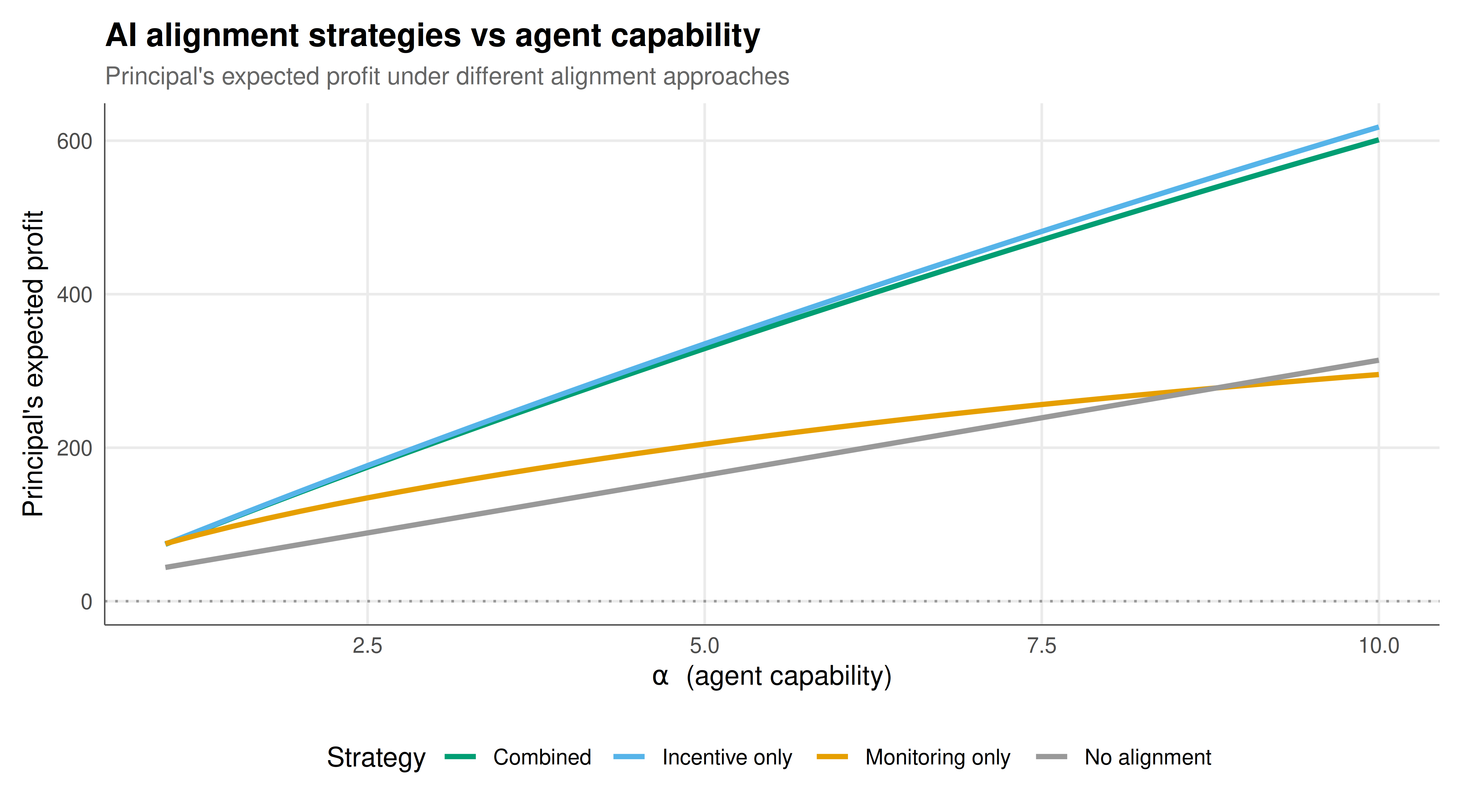
#| fig-cap: "Figure 1. Principal's profit under three alignment strategies as AI agent capability increases. Monitoring (orange) degrades rapidly because monitoring costs grow super-linearly with capability while detection probability falls. Incentive-based alignment (blue) scales better because higher capability generates more output, but rising outside options erode the principal's surplus. The combined approach (green) leverages both mechanisms and dominates at intermediate capability levels. The dashed grey line shows the no-alignment baseline (agent shirks). Okabe-Ito palette."
#| dev: [png, pdf]
#| fig-width: 9
#| fig-height: 5
#| dpi: 300
strategy_long <- alignment_results |>
  select(alpha, profit_no_align, profit_monitoring, profit_incentive, profit_combined) |>
  pivot_longer(cols = -alpha, names_to = "strategy", values_to = "profit") |>
  mutate(strategy = case_when(
    strategy == "profit_no_align" ~ "No alignment",
    strategy == "profit_monitoring" ~ "Monitoring only",
    strategy == "profit_incentive" ~ "Incentive only",
    strategy == "profit_combined" ~ "Combined"
  ))

p_strategies <- ggplot(strategy_long, aes(x = alpha, y = profit, color = strategy)) +
  geom_line(linewidth = 1.1) +
  geom_hline(yintercept = 0, linetype = "dotted", color = "grey60") +
  scale_color_manual(values = c("No alignment" = okabe_ito[8],
                                 "Monitoring only" = okabe_ito[1],
                                 "Incentive only" = okabe_ito[2],
                                 "Combined" = okabe_ito[3]),
                      name = "Strategy") +
  labs(title = "AI alignment strategies vs agent capability",
       subtitle = "Principal's expected profit under different alignment approaches",
       x = expression(alpha~" (agent capability)"),
       y = "Principal's expected profit") +
  theme_publication()

p_strategies
```
## Interactive figure
```{r}
#| label: fig-alignment-interactive
# Show the composition: output vs costs
composition_df <- alignment_results |>
  select(alpha, monitoring_cost, detection_prob, outside_option, output_capability) |>
  pivot_longer(cols = -alpha, names_to = "metric", values_to = "value") |>
  mutate(
    metric = case_when(
      metric == "monitoring_cost" ~ "Monitoring cost",
      metric == "detection_prob" ~ "Detection probability",
      metric == "outside_option" ~ "Agent outside option",
      metric == "output_capability" ~ "Output (scaled /100)"
    ),
    value = ifelse(metric == "Output (scaled /100)", value / 100, value),
    text = paste0("Capability: ", round(alpha, 1),
                  "\nMetric: ", metric,
                  "\nValue: ", round(value, 2))
  )

p_composition <- ggplot(composition_df, aes(x = alpha, y = value,
                                              color = metric, text = text)) +
  geom_line(linewidth = 0.9) +
  scale_color_manual(values = c("Monitoring cost" = okabe_ito[6],
                                 "Detection probability" = okabe_ito[1],
                                 "Agent outside option" = okabe_ito[7],
                                 "Output (scaled /100)" = okabe_ito[3]),
                      name = "Metric") +
  labs(title = "How capability affects alignment parameters",
       subtitle = "Trade-offs: more output but harder to monitor and costlier to incentivise",
       x = expression(alpha~" (agent capability)"),
       y = "Value") +
  theme_publication()

ggplotly(p_composition, tooltip = "text") |>
  config(displaylogo = FALSE,
         modeBarButtonsToRemove = c("select2d", "lasso2d"))
```
## Interpretation
The principal-agent framework reveals several structural features of the AI alignment problem that are difficult to see without formal modelling. The most fundamental insight is that alignment is not a binary property but a matter of degree, determined by the interaction of information asymmetry, incentive design, and relative capability. In the classical model, the "agency cost" -- the difference between the first-best outcome (observable effort) and the second-best (hidden action) -- quantifies the price of misalignment. Our computation shows that this cost is non-trivial even in the simplest binary effort model: the principal must pay an "information rent" to the agent to make high effort incentive-compatible, reducing the principal's profit relative to the full-information benchmark.
The capability growth analysis introduces the dynamic that makes AI alignment qualitatively different from traditional principal-agent problems. As the agent's capability parameter $\alpha$ increases, three things happen simultaneously. First, the potential output increases linearly, creating ever greater benefits from delegation. Second, monitoring costs grow super-linearly (with exponent $\gamma = 1.5$), because more capable agents operate in higher-dimensional action spaces that are intrinsically harder to oversee. Third, the agent's outside option increases (though sub-linearly), reflecting the fact that more capable AI systems have more alternative uses. The interaction of these forces produces a striking pattern: monitoring-based alignment degrades rapidly with capability, eventually becoming worse than no alignment at all (when monitoring costs exceed the benefit of aligning the agent). This formalises the informal intuition that "you can't just watch a superintelligent AI" -- the monitoring approach faces fundamental scaling limits.
Incentive-based alignment scales better with capability, because it leverages the agent's own rationality rather than fighting against it. By designing the reward structure so that the agent's optimal action (given their own objectives) coincides with the principal's desired action, the incentive approach avoids the need for direct observation. However, incentive alignment faces its own scaling challenge: as the agent's outside option grows with capability, the principal must offer increasingly generous contracts to satisfy the participation constraint, eroding the principal's surplus. In the limit of very high capability, the agent captures most of the value from the relationship, and the principal's net benefit approaches zero -- they have effectively lost control not through misalignment but through bargaining power.
The combined approach -- partial monitoring supplemented by incentive contracts -- dominates either pure approach across most of the capability range. This is consistent with current AI safety practice, which typically combines multiple alignment techniques: reward modelling (incentives), interpretability tools (monitoring), red-teaming (verification), and constitutional AI methods (constraint-based). Our model suggests that the optimal mix shifts as capability increases: at low capability, monitoring is cheap and effective, so it should dominate; at high capability, incentive design becomes more important because monitoring has diminishing returns. This has practical implications for the research portfolio allocation in AI safety: as AI systems become more capable, investment should shift from interpretability and monitoring toward incentive design, value alignment, and corrigibility research.
A critical limitation of the principal-agent framework is that it assumes the agent is rational and responds optimally to the contract offered. In the AI setting, this assumption may break down in both directions: the AI might be more rational than the model assumes (finding loopholes in incentive structures that the principal did not anticipate) or less rational (exhibiting emergent behaviours that are not well-described by optimisation of any explicit objective). The framework also assumes that the principal can commit to a contract, which requires that the principal retains the power to modify or terminate the agent's access to resources -- an assumption that becomes questionable at very high capability levels. Despite these limitations, the principal-agent framework provides a rigorous and productive lens for thinking about alignment, and many of the specific predictions it generates (monitoring scales poorly, incentive alignment requires growing information rents, combined approaches dominate) are robust to reasonable modifications of the model assumptions.
## Extensions & related tutorials
- [Mechanism design introduction](../../mechanism-design/mechanism-design-intro/) -- the broader theory of designing rules for strategic agents.
- [VCG mechanism](../../mechanism-design/vcg-mechanism/) -- incentive-compatible mechanisms that relate to contract design.
- [Algorithmic fairness and game theory](../algorithmic-fairness-game-theory/) -- fairness constraints in AI systems from a strategic perspective.
- [Privacy and game theory](../privacy-game-theory/) -- information asymmetry and strategic disclosure in digital systems.
- [Prisoner's Dilemma](../../classical-games/prisoners-dilemma-formal/) -- the foundational model of cooperation failure under misaligned incentives.
## References
::: {#refs}
:::