---
title: "Correlated equilibrium — coordination through shared signals"
description: "Implement Aumann's correlated equilibrium in R via linear programming, compare it with Nash equilibrium, and visualize how a public correlating device expands the set of achievable payoffs."
author: "Raban Heller"
date: 2026-05-08
date-modified: 2026-05-08
categories:
- foundations
- correlated-equilibrium
- equilibrium-concepts
- coordination
keywords: ["correlated equilibrium", "Aumann", "coordination", "linear programming", "Nash equilibrium", "signal"]
labels: ["equilibrium-concepts", "coordination"]
tier: 1
bibliography: ../../../references.bib
vgwort: "TODO_VGWORT_foundations_correlated-equilibrium"
image: thumbnail.png
image-alt: "Correlated equilibrium payoff region containing Nash equilibria as special cases"
citation:
type: webpage
url: https://r-heller.github.io/equilibria/tutorials/foundations/correlated-equilibrium/
license: "CC BY-SA 4.0"
draft: false
has_static_fig: true
has_interactive_fig: true
has_shiny_app: false
---
```{r}
#| label: setup
#| include: false
library(ggplot2)
library(dplyr)
library(tidyr)
library(plotly)
library(lpSolve)
okabe_ito <- c("#E69F00", "#56B4E9", "#009E73", "#F0E442",
"#0072B2", "#D55E00", "#CC79A7", "#999999")
theme_publication <- function(base_size = 12) {
theme_minimal(base_size = base_size) +
theme(plot.title = element_text(size = base_size * 1.2, face = "bold"),
plot.subtitle = element_text(size = base_size * 0.9, color = "grey40"),
axis.line = element_line(color = "grey30", linewidth = 0.3),
panel.grid.minor = element_blank(), legend.position = "bottom",
plot.margin = margin(10, 10, 10, 10))
}
```
## Introduction & motivation
Robert Aumann's 1974 concept of **correlated equilibrium** (CE) generalises Nash equilibrium by allowing players to condition their strategies on a shared random signal — a "correlating device" such as a traffic light, a mediator's recommendation, or a commonly observed public event. The idea is powerful: a mediator privately recommends an action to each player, drawn from a joint distribution over action profiles. If no player can improve their expected payoff by deviating from the recommendation (given what the recommendation reveals about others' likely actions), the distribution is a correlated equilibrium. Every Nash equilibrium is a correlated equilibrium (with independent recommendations), but CE can achieve payoff profiles that no Nash equilibrium reaches — often strictly dominating all Nash equilibria in social welfare. Computationally, while finding Nash equilibria is PPAD-complete (hard), finding a correlated equilibrium that maximises any linear objective is a linear program — solvable in polynomial time. This makes CE both theoretically richer and computationally friendlier than Nash. Aumann's insight formalised an everyday observation: coordination through shared signals (traffic lights, social norms, cultural conventions) allows societies to achieve better outcomes than uncoordinated strategic interaction. This tutorial implements CE computation via LP for 2×2 games in R, compares CE and NE payoff sets for the game of Chicken and Battle of the Sexes, and visualizes how the correlating device expands achievable payoffs.
## Mathematical formulation
For a two-player game with action sets $A_1 = \{1, \ldots, m\}$, $A_2 = \{1, \ldots, n\}$ and payoff matrices $(U, V)$, a **correlated equilibrium** is a probability distribution $p(i,j) \geq 0$ over action profiles such that for all players, no action deviates profitably from the recommendation:
$$
\sum_j p(i,j)[u(i,j) - u(i',j)] \geq 0 \quad \forall i, i' \in A_1
$$
$$
\sum_i p(i,j)[v(i,j) - v(i,j')] \geq 0 \quad \forall j, j' \in A_2
$$
plus $\sum_{i,j} p(i,j) = 1$ and $p(i,j) \geq 0$.
This is a **linear feasibility problem**. To find the welfare-maximising CE, maximise $\sum_{i,j} p(i,j)[u(i,j) + v(i,j)]$ subject to the incentive-compatibility and probability constraints. For a $2 \times 2$ game, there are 4 variables (one per cell) and at most $2 \times 2 \times 2 = 8$ IC constraints.
## R implementation
```{r}
#| label: correlated-equilibrium
# --- Correlated Equilibrium via LP for 2x2 games ---
solve_ce <- function(U, V, objective = "welfare") {
  # U, V: 2x2 payoff matrices (row player, column player)
  # Variables: p11, p12, p21, p22 (row-major)
  m <- nrow(U); n <- ncol(U)
  nvars <- m * n

  # Build IC constraints
  # Row player: for each action i, for each deviation i'≠i:
  #   sum_j p(i,j) * [U(i,j) - U(i',j)] >= 0
  ic_rows <- list()
  for (i in 1:m) {
    for (ip in setdiff(1:m, i)) {
      row <- rep(0, nvars)
      for (j in 1:n) {
        idx <- (i - 1) * n + j
        row[idx] <- U[i, j] - U[ip, j]
      }
      ic_rows <- c(ic_rows, list(row))
    }
  }

  # Column player: for each action j, for each deviation j'≠j:
  #   sum_i p(i,j) * [V(i,j) - V(i,j')] >= 0
  for (j in 1:n) {
    for (jp in setdiff(1:n, j)) {
      row <- rep(0, nvars)
      for (i in 1:m) {
        idx <- (i - 1) * n + j
        row[idx] <- V[i, j] - V[i, jp]
      }
      ic_rows <- c(ic_rows, list(row))
    }
  }

  # Constraint matrix
  A_ic <- do.call(rbind, ic_rows)
  n_ic <- nrow(A_ic)

  # Sum = 1 constraint (equality)
  A_eq <- matrix(rep(1, nvars), nrow = 1)

  # Full constraint matrix
  A_full <- rbind(A_ic, A_eq)
  dir_full <- c(rep(">=", n_ic), "=")
  b_full <- c(rep(0, n_ic), 1)

  # Objective
  if (objective == "welfare") {
    obj <- as.vector(t(U + V))  # maximise social welfare
  } else if (objective == "fair") {
    # Maximise minimum payoff (approximate via equal weights)
    obj <- as.vector(t(U + V))
  }

  result <- lp("max", obj, A_full, dir_full, b_full)

  if (result$status == 0) {
    p <- matrix(result$solution, nrow = m, byrow = TRUE)
    eu1 <- sum(p * U)
    eu2 <- sum(p * V)
    return(list(p = p, eu1 = eu1, eu2 = eu2, welfare = eu1 + eu2, status = "optimal"))
  } else {
    return(list(status = "infeasible"))
  }
}

# --- Game of Chicken ---
U_chicken <- matrix(c(0, -1, 1, -5), nrow = 2, byrow = TRUE)
V_chicken <- matrix(c(0, 1, -1, -5), nrow = 2, byrow = TRUE)
rownames(U_chicken) <- colnames(U_chicken) <- c("Swerve", "Straight")
rownames(V_chicken) <- colnames(V_chicken) <- c("Swerve", "Straight")

ce_chicken <- solve_ce(U_chicken, V_chicken)

cat("=== Game of Chicken ===\n")
cat("Payoff matrix (Row, Col):\n")
for (i in 1:2) for (j in 1:2)
  cat(sprintf("  (%s, %s): (%d, %d)\n", rownames(U_chicken)[i], colnames(U_chicken)[j],
              U_chicken[i,j], V_chicken[i,j]))
cat("\n--- Nash Equilibria ---\n")
cat(" Pure NE 1: (Swerve, Straight) → payoffs (-1, 1)\n")
cat(" Pure NE 2: (Straight, Swerve) → payoffs (1, -1)\n")
cat(" Mixed NE: each Swerves with p = 4/5 → E[payoffs] = (-0.2, -0.2)\n")
cat("\n--- Welfare-Maximising Correlated Equilibrium ---\n")
cat(" Distribution:\n")
for (i in 1:2) for (j in 1:2)
  cat(sprintf("    p(%s, %s) = %.4f\n", rownames(U_chicken)[i], colnames(U_chicken)[j],
              ce_chicken$p[i,j]))
cat(sprintf(" Expected payoffs: (%.3f, %.3f)\n", ce_chicken$eu1, ce_chicken$eu2))
cat(sprintf(" Social welfare: %.3f (vs NE best: 0, NE mixed: -0.4)\n", ce_chicken$welfare))
# --- Battle of the Sexes ---
U_bos <- matrix(c(3, 0, 0, 2), nrow = 2, byrow = TRUE)
V_bos <- matrix(c(2, 0, 0, 3), nrow = 2, byrow = TRUE)
rownames(U_bos) <- colnames(U_bos) <- c("Opera", "Football")

ce_bos <- solve_ce(U_bos, V_bos)

cat("\n=== Battle of the Sexes ===\n")
cat("--- Welfare-Maximising CE ---\n")
for (i in 1:2) for (j in 1:2)
  cat(sprintf("  p(%s, %s) = %.4f\n", rownames(U_bos)[i], colnames(U_bos)[j], ce_bos$p[i,j]))
cat(sprintf("  Expected payoffs: (%.3f, %.3f), welfare = %.3f\n",
            ce_bos$eu1, ce_bos$eu2, ce_bos$welfare))
```
## Static publication-ready figure
```{r}
#| label: fig-ce-payoff-region
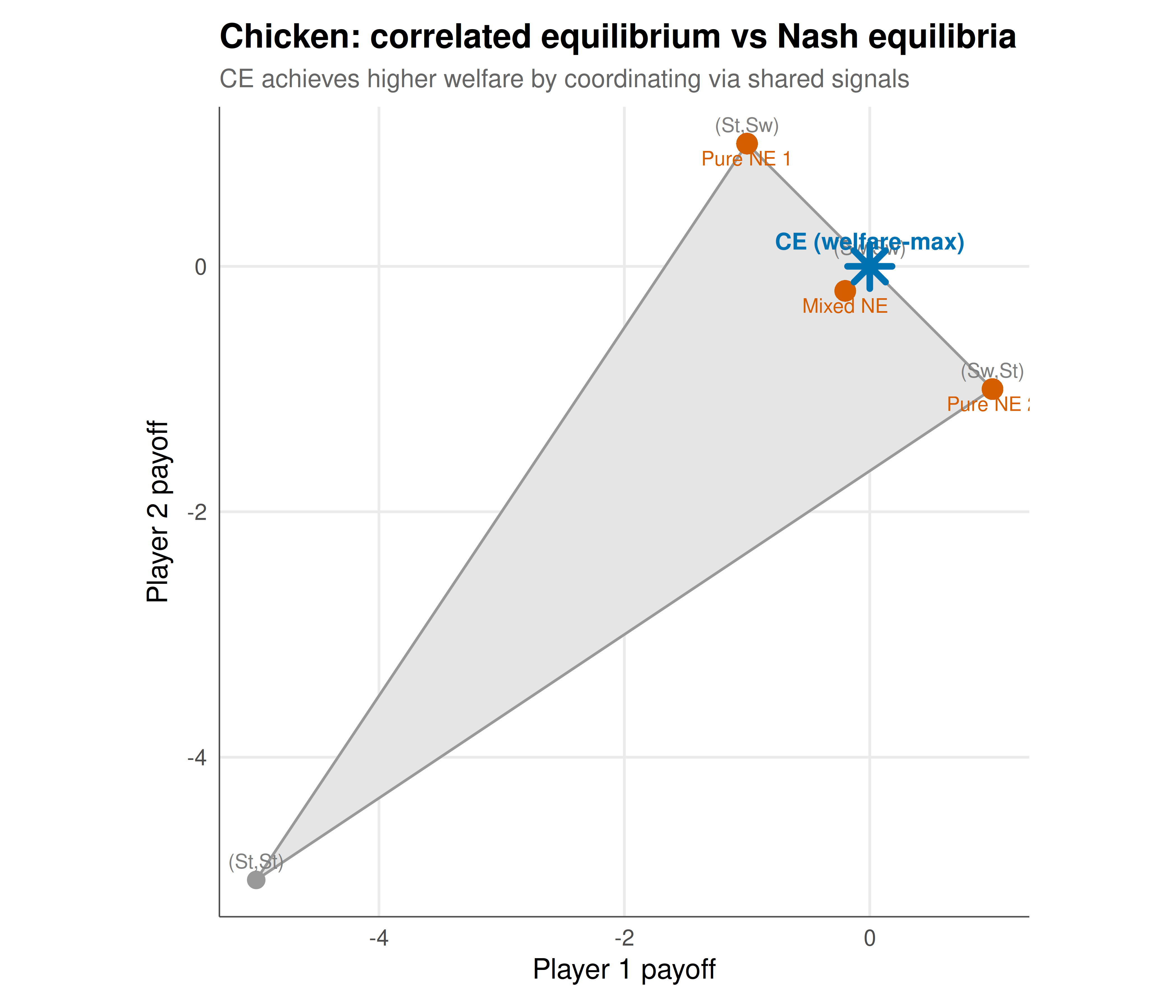
#| fig-cap: "Figure 1. Achievable payoff regions in the Game of Chicken. The convex hull of pure-outcome payoffs (grey polygon) contains all correlated-equilibrium payoffs. Nash equilibria (red points) are special cases — the welfare-maximising CE (blue star) strictly dominates the mixed NE by coordinating players through a shared signal. The CE achieves fairness and efficiency simultaneously by recommending (Swerve, Straight) and (Straight, Swerve) each with probability 1/2, avoiding the disastrous (Straight, Straight) and wasteful (Swerve, Swerve) outcomes. Okabe-Ito palette."
#| dev: [png, pdf]
#| fig-width: 7
#| fig-height: 6
#| dpi: 300
# All pure outcomes in Chicken
outcomes <- tibble(
  u1 = as.vector(U_chicken),
  u2 = as.vector(V_chicken),
  label = c("(Sw,Sw)", "(Sw,St)", "(St,Sw)", "(St,St)")
)

# Convex hull of outcomes = feasible CE payoff region
hull_idx <- chull(outcomes$u1, outcomes$u2)
hull_pts <- outcomes[c(hull_idx, hull_idx[1]), ]

# Nash equilibria
ne_pts <- tibble(
  u1 = c(-1, 1, -0.2),
  u2 = c(1, -1, -0.2),
  label = c("Pure NE 1", "Pure NE 2", "Mixed NE")
)

# CE optimum
ce_pt <- tibble(u1 = ce_chicken$eu1, u2 = ce_chicken$eu2, label = "CE (welfare-max)")

ggplot() +
  geom_polygon(data = hull_pts, aes(x = u1, y = u2), fill = "grey90", color = "grey60") +
  geom_point(data = outcomes, aes(x = u1, y = u2), size = 3, color = okabe_ito[8]) +
  geom_text(data = outcomes, aes(x = u1, y = u2, label = label),
            vjust = -0.8, size = 3, color = "grey50") +
  geom_point(data = ne_pts, aes(x = u1, y = u2), color = okabe_ito[6], size = 4, shape = 16) +
  geom_text(data = ne_pts, aes(x = u1, y = u2, label = label),
            vjust = 1.5, size = 3, color = okabe_ito[6]) +
  geom_point(data = ce_pt, aes(x = u1, y = u2), color = okabe_ito[5], size = 5, shape = 8, stroke = 2) +
  geom_text(data = ce_pt, aes(x = u1, y = u2, label = label),
            vjust = -1, size = 3.5, fontface = "bold", color = okabe_ito[5]) +
  labs(title = "Chicken: correlated equilibrium vs Nash equilibria",
       subtitle = "CE achieves higher welfare by coordinating via shared signals",
       x = "Player 1 payoff", y = "Player 2 payoff") +
  coord_equal() +
  theme_publication()
```
## Interactive figure
```{r}
#| label: fig-ce-exploration
# Explore CE payoff frontier by varying objective weights
weights <- seq(0, 1, by = 0.02)
frontier <- lapply(weights, function(w) {
  # Maximise w*u1 + (1-w)*u2 subject to CE constraints
  obj <- as.vector(t(w * U_chicken + (1 - w) * V_chicken))

  nvars <- 4
  # IC constraints (same as before)
  ic_rows <- list()
  for (i in 1:2) for (ip in setdiff(1:2, i)) {
    row <- rep(0, nvars)
    for (j in 1:2) { idx <- (i-1)*2+j; row[idx] <- U_chicken[i,j] - U_chicken[ip,j] }
    ic_rows <- c(ic_rows, list(row))
  }
  for (j in 1:2) for (jp in setdiff(1:2, j)) {
    row <- rep(0, nvars)
    for (i in 1:2) { idx <- (i-1)*2+j; row[idx] <- V_chicken[i,j] - V_chicken[i,jp] }
    ic_rows <- c(ic_rows, list(row))
  }
  A_ic <- do.call(rbind, ic_rows)
  A_full <- rbind(A_ic, rep(1, 4))
  dir_full <- c(rep(">=", nrow(A_ic)), "=")
  b_full <- c(rep(0, nrow(A_ic)), 1)

  res <- lp("max", obj, A_full, dir_full, b_full)
  p <- matrix(res$solution, nrow = 2, byrow = TRUE)
  tibble(weight = w, eu1 = sum(p * U_chicken), eu2 = sum(p * V_chicken))
}) |> bind_rows() |>
  mutate(text = paste0("Weight on P1: ", round(weight, 2),
                       "\nE[u1] = ", round(eu1, 3),
                       "\nE[u2] = ", round(eu2, 3)))

p_frontier <- ggplot(frontier, aes(x = eu1, y = eu2, text = text)) +
  geom_path(color = okabe_ito[5], linewidth = 1.2) +
  geom_point(data = ne_pts, aes(x = u1, y = u2, text = label),
             color = okabe_ito[6], size = 4) +
  labs(title = "Correlated equilibrium Pareto frontier — Chicken",
       subtitle = "Each point is the CE maximising a different weighted objective",
       x = "Player 1 expected payoff", y = "Player 2 expected payoff") +
  coord_equal() +
  theme_publication()

ggplotly(p_frontier, tooltip = "text") |>
  config(displaylogo = FALSE, modeBarButtonsToRemove = c("select2d", "lasso2d"))
```
## Interpretation
Correlated equilibrium reveals a profound insight about strategic interaction: players can do strictly better by conditioning on a shared signal than by playing independently. In the Game of Chicken, the mixed Nash equilibrium yields expected payoffs of $(-0.2, -0.2)$ — both players are worse off than under any pure NE because the mixing creates a positive probability of the disastrous mutual-Straight outcome. A simple correlating device (a fair coin flip that recommends one player to go Straight and the other to Swerve) achieves payoffs of $(0, 0)$ — eliminating the catastrophic outcome entirely. The key to the CE concept is that following the recommendation is individually rational: if you're told to Swerve, you know the other player was told to go Straight, so Swerving gives you $-1$ while deviating to Straight gives $-5$. No one wants to deviate. The LP formulation makes CE computation tractable even for large games — in stark contrast to Nash equilibrium, where computation is PPAD-hard. The CE Pareto frontier in the interactive figure shows the full range of achievable payoff distributions: by varying the objective weights, the mediator can shift surplus between players while maintaining incentive compatibility. This connection between information design and equilibrium has become central to modern economic theory — from Bergemann and Morris's "Bayes correlated equilibrium" to algorithmic game theory where CE emerges as the natural solution concept for no-regret learning dynamics.
## Extensions & related tutorials
- [Mixed-strategy Nash equilibrium](../nash-equilibrium-mixed/) — the special case without correlation.
- [Battle of the Sexes](../../classical-games/battle-of-the-sexes/) — a coordination game where CE helps.
- [Chicken / Hawk-Dove game](../../classical-games/chicken-hawk-dove/) — the anti-coordination example used here.
- [Zero-sum games and minimax](../zero-sum-minimax-theorem/) — LP methods for game solving.
- [Mechanism design introduction](../../mechanism-design/mechanism-design-intro/) — designing the correlating device optimally.
## References
::: {#refs}
:::